Building a Real-Time Industrial Digital Twin With Apache Flink and Online Machine Learning

Overview

In heavy industrial manufacturing, such as steel hot strip rolling, deterministic physics formulas are the traditional standard for calculating the exact force required to deform a slab of steel. However, these pure physics models share a fatal flaw: they assume a pristine factory state. As physical rollers grind against red-hot steel over hours of production, they experience mechanical wear.

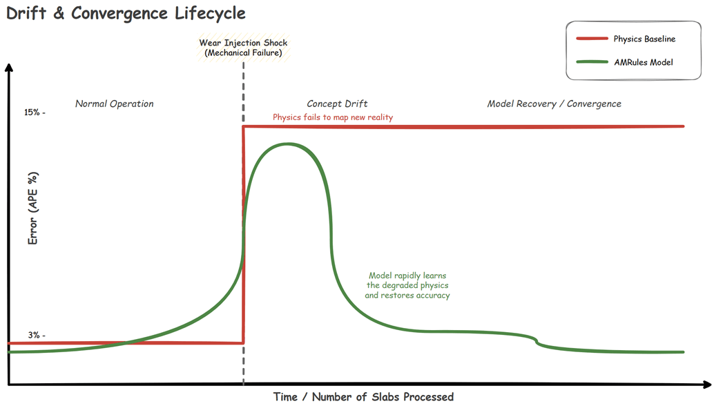
As the machinery degrades, the actual physical force required drifts away from the theoretical prediction. In data science, this is a classic manifestation of Concept Drift.

To tackle this, I recently built a real-time, fault-tolerant Online Machine Learning (OML) pipeline and Digital Twin. By combining Apache Kafka, Apache Flink (written in Kotlin), and the Massive Online Analysis (MOA) framework, the system learns the new physical reality of the worn machinery on the fly, autonomously correcting the physics baseline safely behind a deterministic Shadow Mode router.

Here is an overview of the architecture and the engineering challenges solved along the way. The complete source code for this project, including the Flink stream processor and the Python Digital Twin simulation, is available on GitHub.

Architecture at a Glance

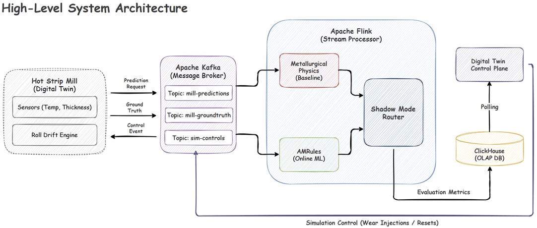
The project is split into three highly decoupled domains:

1. Digital Twin (Python): Utilizing the Dynamic DES Python package, this layer generates synthetic rolling events, applies simulated mechanical wear, calculates theoretical/actual physics, and pushes the data to Kafka.
2. Message Broker (Kafka): Handles the asynchronous, high-throughput streaming of prediction requests and delayed ground-truth target forces.
3. Stream Processor (Flink/Kotlin): The core engine. It aligns asynchronous streams, trains the machine learning models dynamically, evaluates safety guardrails, and sinks metrics to ClickHouse for evaluation in real-time.

Moving data from the Digital Twin through Kafka to Flink looks straightforward in a diagram, but real-world industrial physics and distributed systems are highly complex. To make this pipeline robust enough for the unpredictability of a live factory floor, we had to overcome four major engineering challenges.

Challenges

Taking an online machine learning model out of the lab and deploying it into a live industrial environment introduces a unique set of hurdles. From managing the physical delays of factory sensors to ensuring the model never commands a physically unsafe action, here is a breakdown of the four primary engineering challenges we tackled to make this architecture more robust.

Challenge 1: Asynchronous Industrial Streams

Industrial data streams are inherently asynchronous. The factory floor requests a prediction before the steel enters the rolling stand (Event A), but the ground-truth sensor data confirming the actual required force arrives after the steel is crushed (Event B).

To execute machine learning, these two events must be perfectly joined. However, network latency and partition skew in Kafka mean that these events might arrive out of order.

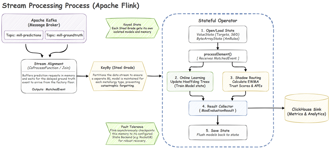
In Flink, this is solved using a KeyedCoProcessFunction. By keying the streams on a composite Slab ID + Pass Number, Flink guarantees both events route to the exact same TaskManager. The EventMatchProcessFunction utilizes Flink’s ValueState to buffer whichever event arrives first. It then registers a processing-time timer (Time-To-Live). If the matching event arrives, they are joined and emitted. If the timer expires (e.g., a physical sensor failure), the orphaned state is safely purged to prevent memory leaks.

Challenge 2: Online Residual Learning

Instead of training a batch model offline on historical data, which would instantly become obsolete the moment the rollers wore down further, the Flink pipeline trains on the continuous stream of slabs using a strict Test-then-Train (prequential) paradigm.

Crucially, the ML models do not predict the absolute rolling force from scratch. Instead, they utilize Residual Learning. They predict the residual error between the theoretical formula and the actual physical force.

To execute this, the pipeline integrates the Java MOA framework. The primary production model is AMRules (Adaptive Model Rules), a streaming rule-learning algorithm. It builds an ensemble of rules that calculate a linear combination of physical attributes, continuously updating weights via the Delta rule.

Unlike static models, AMRules runs an internal Page-Hinkley test to detect sudden physical shocks (like a roller bearing breaking) and instantly prunes obsolete rules, allowing rapid convergence to new physical realities. Furthermore, because ML models require normalized inputs, the pipeline implements Welford’s Online Algorithm in a custom Flink state object to calculate streaming Z-scores on the fly without needing to load full datasets into memory.

Challenge 3: Shadow Mode Router

Industrial Machine Learning cannot operate without strict safety boundaries. A model error that generates excessive rolling force could severely damage a multi-million-dollar rolling stand or create a major production bottleneck in the factory.

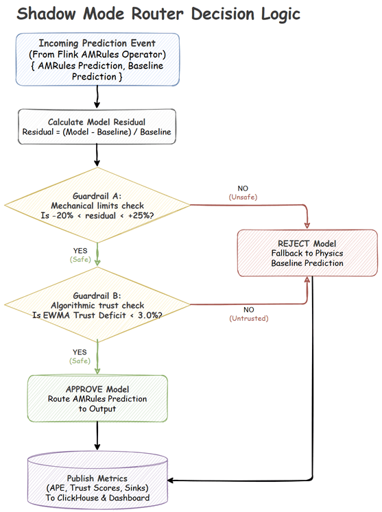
Before any ML-adjusted prediction is allowed to influence the factory floor, it must pass through a deterministic Shadow Mode Router consisting of two guardrails:

1. Stateless Mechanical Limits: Calculates the residual difference between the model’s requested force and the physics baseline. If the model requests a deviation outside of physical safety bounds (e.g., > +25% or < -20%), the prediction is instantly rejected.
2. Stateful Trust Score: Using an Exponentially Weighted Moving Average (EWMA), the router continuously tracks the Absolute Percentage Error (APE) of both the model and the pure physics baseline. If the model’s average error trails the physics baseline by a defined “Trust Deficit” margin, it is benched.

If either guardrail is triggered, the router safely falls back to the deterministic Physics Baseline. The ML model continues to train in the background (Shadow Mode) until it re-learns the physical reality, improves its EWMA trust score, and is autonomously promoted back to active control.

Challenge 4: Checkpointing Complex ML State

For Flink to provide exactly-once processing guarantees, it must asynchronously snapshot the state of operators to a durable backend like RocksDB.

While simple tracking states serialize perfectly into basic Flink ValueState<Double>, the AMRules model is a deeply complex, dynamic tree structure. Allowing Flink’s default Kryo serializers to traverse this massive object graph during checkpointing causes severe performance degradation and frequent serialization crashes.

To bypass this, the MoaEvaluationProcessFunction interacts with the MOA model as a standard Java object in memory for high-performance execution. However, upon every state update, it manually serializes the model into a raw byte array (ValueState<ByteArray>) using Java’s native ObjectOutputStream. When Flink triggers a checkpoint, it simply flushes these pre-serialized byte arrays to disk. Upon recovery, Flink deserializes the bytes, instantly restoring the exact computational brain-state of the algorithm.

System in Action

You can easily spin up the entire architecture locally to see the system in action. The project repository includes a complete Docker Compose environment that provisions Kafka, Flink, and ClickHouse.

To get started, simply clone the repository, build the Flink application using the provided Gradle wrapper, and bring up the infrastructure. Once the environment is running, you can launch the Python-based data generator to simulate the steel rolling process and open the NiceGUI control dashboard to monitor the machine learning metrics in real-time.

For detailed, step-by-step instructions on cloning the repository, configuring licenses, and deploying the Flink job, refer to the Getting Started section in the repository.

Simulation Scenarios

Using the NiceGUI Dashboard, you can actively manipulate the physical state of the Digital Twin to observe the Flink pipeline’s reaction in real-time.

Here is how the pipeline handles different industrial scenarios:

Abrupt Drift (Mechanical Shock)

Simulates a sudden mechanical failure (e.g., a roller bearing breaking), instantly altering the physics of the mill.

• Simulation Settings: Trigger Abrupt Shock (Wear Level: 60.0).
• Observation: The pure physics baseline error instantly spikes and remains high (often >10% APE) because the physical reality no longer matches the math. The AMRules model initially spikes alongside it, but its Page-Hinkley change detector immediately drops obsolete rules, allowing it to rapidly converge back to lower error as it learns the new broken state.

Gradual Drift (Standard Wear)

Simulates the continuous, bi-directional cycle of slow roller degradation and subsequent maintenance recovery over hours of production.

• Simulation Settings: Gradual Wear (Step Size: 5.0 units, Frequency: 30 seconds).
• Observation: The physics baseline error slowly and persistently creeps upward/download over time (e.g. ranging from 2% to 7% APE) as the wear level drifts gradually. The AMRules model gracefully tracks this changing reality, updating its linear weights incrementally to maintain a smooth error rate.

No Drift (Pristine State)

Simulates a pristine factory state, such as immediately after a maintenance shift replaces the rollers.

• Simulation Settings: Wear Level: 0.0.
• Observation: The physical reality of the factory floor perfectly aligns with the deterministic mathematical formulas. The physics baseline maintains a highly accurate, near-zero error rate (< 0.3% APE). AMRules remains stable under this condition.

Conclusion

Combining Apache Flink with Online Machine Learning bridges the gap between theoretical physics and the harsh reality of a degrading factory floor. To make this safe and effective, the architecture relies on three core ideas: predicting residual errors instead of absolute forces, isolating models by product line to prevent forgetting, and enforcing strict safety guardrails. Together, these techniques ensure that heavy machinery operates optimally, even as it breaks down over time.

You can explore the complete codebase, run the simulation locally, and dive deeper into the architecture on the project’s GitHub repository.