This is the first article about tree based methods using R. Carseats data in the chapter 8 lab of ISLR is used to perform classification analysis. Unlike the lab example, the rpart package is used to fit the CART model on the data and the caret package is used for tuning the pruning parameter (cp).
The bold-cased sections of the tutorial are covered in this article.
- Visualizations
- Pre-Processing
- Data Splitting
- Miscellaneous Model Functions
- Model Training and Tuning
- Using Custom Models
- Variable Importance
- Feature Selection: RFE, Filters, GA, SA
- Other Functions
- Parallel Processing
- Adaptive Resampling
The pruning parameter in the rpart package is scaled so that its values are from 0 to 1. Specifically the formula is
$$ R_{cp}\left(T\right)\equiv R\left(T\right) + cp*|T|*R\left(T_{1}\right) $$
where $$T_{1}$$ is the tree with no splits, $$\mid T\mid$$ is the number of splits for a tree and R is the risk.
Due to the inclusion of $$R\left(T_{1}\right)$$, when cp=1, the tree will result in no splits while it is not pruned when cp=0. On the other hand, in the original setup without the term, the pruning parameter ($$\alpha$$) can range from 0 to infinity.
Let’s get started.
The following packages are used.
1library(dplyr) # data minipulation
2library(rpart) # fit tree
3library(rpart.plot) # plot tree
4library(caret) # tune model
Carseats data is created as following while the response (Sales) is converted into a binary variable.
1require(ISLR)
2data(Carseats)
3Carseats = Carseats %>%
4  mutate(High=factor(ifelse(Sales<=8,"No","High"),labels=c("High","No")))
5# structure of predictors
6str(subset(Carseats,select=c(-High,-Sales)))
## 'data.frame':	400 obs. of  10 variables:
##  $ CompPrice  : num  138 111 113 117 141 124 115 136 132 132 ...
##  $ Income     : num  73 48 35 100 64 113 105 81 110 113 ...
##  $ Advertising: num  11 16 10 4 3 13 0 15 0 0 ...
##  $ Population : num  276 260 269 466 340 501 45 425 108 131 ...
##  $ Price      : num  120 83 80 97 128 72 108 120 124 124 ...
##  $ ShelveLoc  : Factor w/ 3 levels "Bad","Good","Medium": 1 2 3 3 1 1 3 2 3 3 ...
##  $ Age        : num  42 65 59 55 38 78 71 67 76 76 ...
##  $ Education  : num  17 10 12 14 13 16 15 10 10 17 ...
##  $ Urban      : Factor w/ 2 levels "No","Yes": 2 2 2 2 2 1 2 2 1 1 ...
##  $ US         : Factor w/ 2 levels "No","Yes": 2 2 2 2 1 2 1 2 1 2 ...
1# classification response summary
2with(Carseats,table(High))
## High
## High   No
##  164  236
1with(Carseats,table(High) / length(High))
## High
## High   No
## 0.41 0.59
The train and test data sets are split using createDataPartition().
1## Data Splitting
2set.seed(1237)
3trainIndex.cl = createDataPartition(Carseats$High, p=.8, list=FALSE, times=1)
4trainData.cl = subset(Carseats, select=c(-Sales))[trainIndex.cl,]
5testData.cl = subset(Carseats, select=c(-Sales))[-trainIndex.cl,]
Stratify sampling is performed by default.
1# training response summary
2with(trainData.cl,table(High))
## High
## High   No
##  132  189
1with(trainData.cl,table(High) / length(High))
## High
##     High       No
## 0.411215 0.588785
1# test response summary
2with(testData.cl,table(High))
## High
## High   No
##   32   47
1with(testData.cl,table(High) / length(High))
## High
##      High        No
## 0.4050633 0.5949367
The following resampling strategies are considered: cross-validation, repeated cross-validation and bootstrap.
1## train control
2trControl.cv = trainControl(method="cv",number=10)
3trControl.recv = trainControl(method="repeatedcv",number=10,repeats=5)
4trControl.boot = trainControl(method="boot",number=50)
There are two methods in the caret package: rpart and repart2. The first method allows the pruning parameter to be tuned. The tune grid is not set up explicitly and it is adjusted by tuneLength - equally spaced cp values are created from 0 to 0.3 in the package.
 1set.seed(12357)
 2fit.cl.cv = train(High ~ .
 3                  ,data=trainData.cl
 4                  ,method="rpart"
 5                  ,tuneLength=20
 6                  ,trControl=trControl.cv)
 7
 8fit.cl.recv = train(High ~ .
 9                    ,data=trainData.cl
10                    ,method="rpart"
11                    ,tuneLength=20
12                    ,trControl=trControl.recv)
13
14fit.cl.boot = train(High ~ .
15                    ,data=trainData.cl
16                    ,method="rpart"
17                    ,tuneLength=20
18                    ,trControl=trControl.boot)
Repeated cross-validation and bootstrap produce the same best tuned cp value while cross-validation returns a higher value.
1# results at best tuned cp
2subset(fit.cl.cv$results,subset=cp==fit.cl.cv$bestTune$cp)
##           cp  Accuracy     Kappa AccuracySD   KappaSD
## 3 0.03110048 0.7382148 0.4395888 0.06115425 0.1355713
1subset(fit.cl.recv$results,subset=cp==fit.cl.recv$bestTune$cp)
##           cp  Accuracy    Kappa AccuracySD   KappaSD
## 2 0.01555024 0.7384537 0.456367 0.08602102 0.1821254
1subset(fit.cl.boot$results,subset=cp==fit.cl.boot$bestTune$cp)
##           cp  Accuracy     Kappa AccuracySD    KappaSD
## 2 0.01555024 0.7178692 0.4163337 0.04207806 0.08445416
The one from repeated cross-validation is taken to fit to the entire training data.
Updated on Feb 10, 2015
- As a value of cp is entered in
rpart(), the function fits the model up to the value and takes the result. Therefore it produces a pruned tree. - If it is not set or set to be a low value (eg, 0), pruning can be done using the
prune()function.
1## refit the model to the entire training data
2cp.cl = fit.cl.recv$bestTune$cp
3fit.cl = rpart(High ~ ., data=trainData.cl, control=rpart.control(cp=cp.cl))
4
5# Updated on Feb 10, 2015
6# prune if cp not set or too low
7# fit.cl = prune(tree=fit.cl, cp=cp.cl)
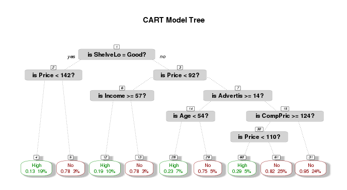
The resulting tree is shown as following. The plot shows expected losses and node probabilities in the final nodes. For example, the leftmost node has
- expected loss of 0.13 (= 8/60 (0.13333))
- node probability of 19% (= 60/321)
 1# plot tree
 2cols <- ifelse(fit.cl$frame$yval == 1,"green4","darkred") # green if high
 3prp(fit.cl
 4    ,main="CART model tree"
 5    ,extra=106           # display prob of survival and percent of obs
 6    ,nn=TRUE             # display the node numbers
 7    ,fallen.leaves=TRUE  # put the leaves on the bottom of the page
 8    ,branch=.5           # change angle of branch lines
 9    ,faclen=0            # do not abbreviate factor levels
10    ,trace=1             # print the automatically calculated cex
11    ,shadow.col="gray"   # shadows under the leaves
12    ,branch.lty=3        # draw branches using dotted lines
13    ,split.cex=1.2       # make the split text larger than the node text
14    ,split.prefix="is "  # put "is " before split text
15    ,split.suffix="?"    # put "?" after split text
16    ,col=cols, border.col=cols   # green if survived
17    ,split.box.col="lightgray"   # lightgray split boxes (default is white)
18    ,split.border.col="darkgray" # darkgray border on split boxes
19    ,split.round=.5)
## cex 0.7 xlim c(0, 1) ylim c(-0.1, 1.1)
The fitted model is applied to the test data.
1## apply to the test data
2pre.cl = predict(fit.cl, newdata=testData.cl, type="class")
3
4# confusion matrix
5cMat.cl = table(data.frame(response=pre.cl,truth=testData.cl$High))
6cMat.cl
##         truth
## response High No
##     High   21  4
##     No     11 43
1# mean misclassification error
2mmse.cl = 1 - sum(diag(cMat.cl))/sum(cMat.cl)
3mmse.cl
## [1] 0.1898734
More models are going to be implemented/compared in the subsequent articles.
Comments