In the previous article (Tree Based Methods in R - Part I), a decision tree is created on the Carseats data which is in the chapter 8 lab of ISLR. In that article, potentially asymetric costs due to misclassification are not taken into account. When unbalance between false positive and false negative can have a significant impact, it can be explicitly adjusted either by altering prior (or empirical) probabilities or by adding a loss matrix.
A comprehensive summary of this topic, as illustrated in Berk (2008), is shown below.
…when the CART solution is determined solely by the data, the prior distribution is empirically determined, and the costs in the loss matrix of all classification errors are the same. Costs are being assigned even if the data analyst makes no conscious decision about them. Should the balance of false negatives to false positives that results be unsatisfactory, that balance can be changed. Either the costs in the loss matrix can be directly altered, leaving the prior distribution to be empirically determined, or the prior distribution can be altered leaving the default costs untouched. Much of the software currently available makes it easier to change the prior in the binary response case. When there are more than two response categories, it will usually be easier in practice to change the costs in the loss matrix directly.
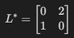
In this article, cost-sensitive classification is implemented, assuming that misclassifying the High class is twice as expensive, both by altering the priors and by adjusting the loss matrix.
The following loss matrix is implemented.
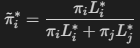
The corresponding altered priors can be obtained by
The bold-cased sections of the tutorial of the caret package are covered in this article.
- Visualizations
- Pre-Processing
- Data Splitting
- Miscellaneous Model Functions
- Model Training and Tuning
- Using Custom Models
- Variable Importance
- Feature Selection: RFE, Filters, GA, SA
- Other Functions
- Parallel Processing
- Adaptive Resampling
Let’s get started.
The following packages are used.
1library(dplyr) # data minipulation
2library(rpart) # fit tree
3library(rpart.plot) # plot tree
4library(caret) # tune model
Carseats data is created as following while the response (Sales) is converted into a binary variable.
1require(ISLR)
2data(Carseats)
3Carseats = Carseats %>%
4  mutate(High=factor(ifelse(Sales<=8,"No","High"),labels=c("High","No")))
5# structure of predictors
6str(subset(Carseats,select=c(-High,-Sales)))
## 'data.frame':	400 obs. of  10 variables:
##  $ CompPrice  : num  138 111 113 117 141 124 115 136 132 132 ...
##  $ Income     : num  73 48 35 100 64 113 105 81 110 113 ...
##  $ Advertising: num  11 16 10 4 3 13 0 15 0 0 ...
##  $ Population : num  276 260 269 466 340 501 45 425 108 131 ...
##  $ Price      : num  120 83 80 97 128 72 108 120 124 124 ...
##  $ ShelveLoc  : Factor w/ 3 levels "Bad","Good","Medium": 1 2 3 3 1 1 3 2 3 3 ...
##  $ Age        : num  42 65 59 55 38 78 71 67 76 76 ...
##  $ Education  : num  17 10 12 14 13 16 15 10 10 17 ...
##  $ Urban      : Factor w/ 2 levels "No","Yes": 2 2 2 2 2 1 2 2 1 1 ...
##  $ US         : Factor w/ 2 levels "No","Yes": 2 2 2 2 1 2 1 2 1 2 ...
1# classification response summary
2res.summary = with(Carseats,rbind(table(High),table(High)/length(High)))
3res.summary
##        High     No
## [1,] 164.00 236.00
## [2,]   0.41   0.59
The train and test data sets are split using createDataPartition().
1# split data
2set.seed(1237)
3trainIndex = createDataPartition(Carseats$High, p=.8, list=FALSE, times=1)
4trainData = subset(Carseats, select=c(-Sales))[trainIndex,]
5testData = subset(Carseats, select=c(-Sales))[-trainIndex,]
6
7# response summary
8train.res.summary = with(trainData,rbind(table(High),table(High)/length(High)))
9test.res.summary = with(testData,rbind(table(High),table(High)/length(High)))
5 repeats of 10-fold cross validation is set up.
1# set up train control
2trControl = trainControl(method="repeatedcv",number=10,repeats=5)
Rather than tuning the complexity parameter (cp) using the built-in tuneLength, a grid is created. At first, it was intended to use this grid together with altered priors in the expand.grid() function of the caret package as rpart() has an argument named parms to enter altered priors (prior) or a loss matrix (loss) as a list. Later, however, it was found that the function does not accept an argument if it is not set as a tuning parameter. Therefore cp is not tuned when each of parms values is modified. (Although it is not considered in this article, the mlr package seems to support cost sensitive classification by adding a loss matrix as can be checked here)
 1# generate tune grid
 2cpGrid = function(start,end,len) {
 3  inc = if(end > start) (end-start)/len else 0
 4  # update grid
 5  if(inc > 0) {
 6    grid = c(start)
 7    while(start < end) {
 8      start = start + inc
 9      grid = c(grid,start)
10    }
11  } else {
12    message("start > end, default cp value is taken")
13    grid = c(0.1)
14  }
15  grid
16}
17
18grid = expand.grid(cp=cpGrid(0,0.3,20))
The default model is fit below.
 1# train model with equal cost
 2set.seed(12357)
 3mod.eq.cost = train(High ~ .
 4                      ,data=trainData
 5                      ,method="rpart"
 6                      ,tuneGrid=grid
 7                      ,trControl=trControl)
 8
 9# select results at best tuned cp
10subset(mod.eq.cost$results,subset=cp==mod.eq.cost$bestTune$cp)
##      cp  Accuracy     Kappa AccuracySD   KappaSD
## 2 0.015 0.7303501 0.4383323  0.0836073 0.1743789
The model is refit with the tuned cp value.
1# refit the model to the entire training data
2cp = mod.eq.cost$bestTune$cp
3mod.eq.cost = rpart(High ~ ., data=trainData, control=rpart.control(cp=cp))
Confusion matrices are obtained from both the training and test data sets. Here the matrices are transposed to the previous article and this is to keep the same structure as used in Berk (2008) - the source of getUpdatedCM() can be found in this gist.
The model error means how successful fitting or prediction is on each class given data and it is shown that the High class is more misclassified. The use error is to see how useful the model is given fitted or predicted values. It is also found that misclassification of the High class becomes worse when the model is applied to the test data.
1source("src/mlUtils.R")
2fit.eq.cost = predict(mod.eq.cost, type="class")
3fit.cm.eq.cost = table(data.frame(actual=trainData$High,response=fit.eq.cost))
4fit.cm.eq.cost = getUpdatedCM(cm=fit.cm.eq.cost, type="Fitted")
5fit.cm.eq.cost
##              Fitted: High Fitted: No Model Error
## Actual: High       106.00      26.00        0.20
## Actual: No          24.00     165.00        0.13
## Use Error            0.18       0.14        0.16
1pred.eq.cost = predict(mod.eq.cost, newdata=testData, type="class")
2pred.cm.eq.cost = table(data.frame(actual=testData$High,response=pred.eq.cost))
3pred.cm.eq.cost = getUpdatedCM(pred.cm.eq.cost)
4pred.cm.eq.cost
##              Pred: High Pred: No Model Error
## Actual: High      21.00     11.0        0.34
## Actual: No         4.00     43.0        0.09
## Use Error          0.16      0.2        0.19
As mentioned earlier, either althered priors or a loss matrix can be entered into rpart(). They are created below.
1# update prior probabilities
2costs = c(2,1)
3train.res.summary
##            High         No
## [1,] 132.000000 189.000000
## [2,]   0.411215   0.588785
1prior.w.weight = c(train.res.summary[2,1] * costs[1]
2                   ,train.res.summary[2,2] * costs[2])
3priorUp = c(prior.w.weight[1]/sum(prior.w.weight)
4            ,prior.w.weight[2]/sum(prior.w.weight))
5priorUp
##      High        No
## 0.5827815 0.4172185
1# loss matrix
2loss.mat = matrix(c(0,2,1,0),nrow=2,byrow=TRUE)
3loss.mat
##      [,1] [,2]
## [1,]    0    2
## [2,]    1    0
Both will deliver the same outcome.
1# refit the model with the updated priors
2# fit with updated prior
3mod.uq.cost = rpart(High ~ ., data=trainData, parms=list(prior=priorUp), control=rpart.control(cp=cp))
4
5# fit with loss matrix
6# mod.uq.cost = rpart(High ~ ., data=trainData, parms=list(loss=loss.mat), control=rpart.control(cp=cp))
Confusion matrices are obtained again. It is shown that more values are classified as the High class. Note that, although the overall misclassification error is increased, it does not reflect costs. In a situation, the cost adjusted CART may be more beneficial.
1fit.cm.eq.cost
##              Fitted: High Fitted: No Model Error
## Actual: High       106.00      26.00        0.20
## Actual: No          24.00     165.00        0.13
## Use Error            0.18       0.14        0.16
1fit.uq.cost = predict(mod.uq.cost, type="class")
2fit.cm.uq.cost = table(data.frame(actual=trainData$High,response=fit.uq.cost))
3fit.cm.uq.cost = getUpdatedCM(fit.cm.uq.cost, type="Fitted")
4fit.cm.uq.cost
##              Fitted: High Fitted: No Model Error
## Actual: High       123.00       9.00        0.07
## Actual: No          44.00     145.00        0.23
## Use Error            0.26       0.06        0.17
1pred.cm.eq.cost
##              Pred: High Pred: No Model Error
## Actual: High      21.00     11.0        0.34
## Actual: No         4.00     43.0        0.09
## Use Error          0.16      0.2        0.19
1pred.uq.cost = predict(mod.uq.cost, newdata=testData, type="class")
2pred.cm.uq.cost = table(data.frame(actual=testData$High,response=pred.uq.cost))
3pred.cm.uq.cost = getUpdatedCM(pred.cm.uq.cost)
4pred.cm.uq.cost
##              Pred: High Pred: No Model Error
## Actual: High      26.00     6.00        0.19
## Actual: No        14.00    33.00        0.30
## Use Error          0.35     0.15        0.25
Comments