While classification tasks are implemented in the last two articles (Part I and Part II), a regression task is the topic of this article. While the caret package selects the tuning parameter (cp) that minimizes the error (RMSE), the rpart packages recommends the 1-SE rule, which selects the smallest tree within 1 standard error of the minimum cross validation error (xerror). The models with 2 complexity parameters that are suggested by the packages are compared.
The bold-cased sections of the tutorial of the caret package are covered in this article.
- Visualizations
- Pre-Processing
- Data Splitting
- Miscellaneous Model Functions
- Model Training and Tuning
- Using Custom Models
- Variable Importance
- Feature Selection: RFE, Filters, GA, SA
- Other Functions
- Parallel Processing
- Adaptive Resampling
Let’s get started.
The following packages are used.
1library(knitr)
2library(dplyr)
3library(ggplot2)
4library(grid)
5library(gridExtra)
6library(rpart)
7library(rpart.plot)
8library(caret)
The Carseats data from the ISLR package is used - a dummy variable (High) is created from Sales for classification. Note that the order of the labels is changed from the previous articles for comparison with the regression model.
1## data
2require(ISLR)
3data(Carseats)
4# label order changed (No=1)
5Carseats = Carseats %>%
6  mutate(High=factor(ifelse(Sales<=8,"No","High"),labels=c("No","High")))
7# structure of predictors
8str(subset(Carseats,select=c(-High,-Sales)))
## 'data.frame':	400 obs. of  10 variables:
##  $ CompPrice  : num  138 111 113 117 141 124 115 136 132 132 ...
##  $ Income     : num  73 48 35 100 64 113 105 81 110 113 ...
##  $ Advertising: num  11 16 10 4 3 13 0 15 0 0 ...
##  $ Population : num  276 260 269 466 340 501 45 425 108 131 ...
##  $ Price      : num  120 83 80 97 128 72 108 120 124 124 ...
##  $ ShelveLoc  : Factor w/ 3 levels "Bad","Good","Medium": 1 2 3 3 1 1 3 2 3 3 ...
##  $ Age        : num  42 65 59 55 38 78 71 67 76 76 ...
##  $ Education  : num  17 10 12 14 13 16 15 10 10 17 ...
##  $ Urban      : Factor w/ 2 levels "No","Yes": 2 2 2 2 2 1 2 2 1 1 ...
##  $ US         : Factor w/ 2 levels "No","Yes": 2 2 2 2 1 2 1 2 1 2 ...
1# response summaries
2res.cl.summary = with(Carseats,rbind(table(High),table(High)/length(High)))
3res.cl.summary
##          No   High
## [1,] 164.00 236.00
## [2,]   0.41   0.59
1res.reg.summary = summary(Carseats$Sales)
2res.reg.summary
##    Min. 1st Qu.  Median    Mean 3rd Qu.    Max.
##   0.000   5.390   7.490   7.496   9.320  16.270
The data is split as following.
 1## split data
 2set.seed(1237)
 3trainIndex = createDataPartition(Carseats$High, p=.8, list=FALSE, times=1)
 4# classification
 5trainData.cl = subset(Carseats, select=c(-Sales))[trainIndex,]
 6testData.cl = subset(Carseats, select=c(-Sales))[-trainIndex,]
 7# regression
 8trainData.reg = subset(Carseats, select=c(-High))[trainIndex,]
 9testData.reg = subset(Carseats, select=c(-High))[-trainIndex,]
10
11# response summary
12train.res.cl.summary = with(trainData.cl,rbind(table(High),table(High)/length(High)))
13test.res.cl.summary = with(testData.cl,rbind(table(High),table(High)/length(High)))
14
15train.res.reg.summary = summary(trainData.reg$Sales)
16test.res.reg.summary = summary(testData.reg$Sales)
1## train model
2# set up train control
3trControl = trainControl(method="repeatedcv",number=10,repeats=5)
Having 5 times of 10-fold cross-validation set above, both the CART is fit as both classification and regression tasks.
1# classification
2set.seed(12357)
3mod.cl = train(High ~ .
4               ,data=trainData.cl
5               ,method="rpart"
6               ,tuneLength=20
7               ,trControl=trControl)
Note that the package developer informs that, in spite of the warning messages, the function fits the training data without a problem so that the outcome can be relied upon (Link). Note that the criterion is selecting the cp that has the lowest RMSE.
1# regression - caret
2set.seed(12357)
3mod.reg.caret = train(Sales ~ .
4                      ,data=trainData.reg
5                      ,method="rpart"
6                      ,tuneLength=20
7                      ,trControl=trControl)
## Warning in nominalTrainWorkflow(x = x, y = y, wts = weights, info =
## trainInfo, : There were missing values in resampled performance measures.
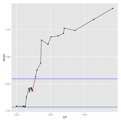
For comparison, the data is fit using rpart() where the cp value is set to 0. This cp value results in an unpruned tree and cp can be selected by the 1-SE rule, which selects the smallest tree within 1 standard error of the minimum cross validation error (xerror), which is recommended by the package. Note that a custom function (bestParam()) is used to search the best parameter by the 1-SE rule and the source can be found here.
1# regression - rpart
2source("src/mlUtils.R")
3set.seed(12357)
4mod.reg.rpart = rpart(Sales ~ ., data=trainData.reg, control=rpart.control(cp=0))
5mod.reg.rpart.param = bestParam(mod.reg.rpart$cptable,"CP","xerror","xstd")
6mod.reg.rpart.param
##             lowest        best
## param  0.004852267 0.009349806
## error  0.585672544 0.610102155
## errStd 0.041710792 0.041305185
If it is necessary to apply the 1-SE rule on the result by the caret package, the bestParam() can be used by setting isDesc to be FALSE. The result is shown below as reference.
1mod.reg.caret.param = bestParam(mod.reg.caret$results,"cp","RMSE","RMSESD",isDesc=FALSE)
2mod.reg.caret.param
##            lowest       best
## param  0.00828502 0.05661803
## error  2.23430550 2.38751487
## errStd 0.23521777 0.27267509
A graphical display of the best cp is shown below.
 1# plot best CP
 2df = as.data.frame(mod.reg.rpart$cptable)
 3best = bestParam(mod.reg.rpart$cptable,"CP","xerror","xstd")
 4ubound = ifelse(best[2,1]+best[3,1]>max(df$xerror),max(df$xerror),best[2,1]+best[3,1])
 5lbound = ifelse(best[2,1]-best[3,1]<min(df$xerror),min(df$xerror),best[2,1]-best[3,1])
 6
 7ggplot(data=df[3:nrow(df),], aes(x=CP,y=xerror)) +
 8  geom_line() + geom_point() +
 9  geom_abline(intercept=ubound,slope=0, color="blue") +
10  geom_abline(intercept=lbound,slope=0, color="blue") +
11  geom_point(aes(x=best[1,2],y=best[2,2]),color="red",size=3)
The best cp values for each of the models are shown below
1## show best tuned cp
2# classification
3subset(mod.cl$results,subset=cp==mod.cl$bestTune$cp)
##   cp  Accuracy     Kappa AccuracySD  KappaSD
## 1  0 0.7262793 0.4340102 0.07561158 0.153978
1# regression - caret
2subset(mod.reg.caret$results,subset=cp==mod.reg.caret$bestTune$cp)
##           cp     RMSE  Rsquared    RMSESD RsquaredSD
## 1 0.00828502 2.234305 0.4342292 0.2352178  0.1025357
1# regression - rpart
2mod.reg.rpart.summary = data.frame(t(mod.reg.rpart.param[,2]))
3colnames(mod.reg.rpart.summary) = c("CP","xerror","xstd")
4mod.reg.rpart.summary
##            CP    xerror       xstd
## 1 0.009349806 0.6101022 0.04130518
The training data is refit with the best cp values.
 1## refit the model to the entire training data
 2# classification
 3cp.cl = mod.cl$bestTune$cp
 4mod.cl = rpart(High ~ ., data=trainData.cl, control=rpart.control(cp=cp.cl))
 5
 6# regression - caret
 7cp.reg.caret = mod.reg.caret$bestTune$cp
 8mod.reg.caret = rpart(Sales ~ ., data=trainData.reg, control=rpart.control(cp=cp.reg.caret))
 9
10# regression - rpart
11cp.reg.rpart = mod.reg.rpart.param[1,2]
12mod.reg.rpart = rpart(Sales ~ ., data=trainData.reg, control=rpart.control(cp=cp.reg.rpart))
Initially it was planned to compare the regression model to the classification model. Specifically, as the response is converted as a binary variable and the break is at the value of 8.0, it is possible to create a regression version of confusion matrix by splitting the data at the equivalent percentile, which is about 0.59 in this data. Then the outcomes can be compared. However it turns out that they cannot be compared directly as the regression outcome is too good as shown below. Note updateCM() and regCM() are custom functions and their sources can be found here.
 1## generate confusion matrix on training data
 2# fit models
 3fit.cl = predict(mod.cl, type="class")
 4fit.reg.caret = predict(mod.reg.caret)
 5fit.reg.rpart = predict(mod.reg.rpart)
 6
 7# classification
 8# percentile that Sales is divided by No and High
 9eqPercentile = with(trainData.reg,length(Sales[Sales<=8])/length(Sales))
10
11# classification
12fit.cl.cm = table(data.frame(actual=trainData.cl$High,response=fit.cl))
13fit.cl.cm = updateCM(fit.cl.cm,type="Fitted")
14fit.cl.cm
##              Fitted: No Fitted: High Model Error
## actual: No       111.00        21.00        0.16
## actual: High      26.00       163.00        0.14
## Use Error          0.19         0.11        0.15
1# regression with equal percentile is not comparable
2probs = eqPercentile
3fit.reg.caret.cm = regCM(trainData.reg$Sales, fit.reg.caret, probs=probs, type="Fitted")
4fit.reg.caret.cm
##              Fitted: 59%- Fitted: 59%+ Model Error
## actual: 59%-          185         4.00        0.02
## actual: 59%+            0       132.00        0.00
## Use Error               0         0.03        0.01
As it is not easy to compare the classification and regression models directly, only the 2 regression models are compared from now on. At first, the regression version of confusion matrices are compared by every 20th percentile followed by the residual mean sqaured error (RMSE) values.
1# regression with selected percentiles
2probs = seq(0.2,0.8,0.2)
3
4# regression - caret
5# caret produces a better outcome on training data - note lower cp
6fit.reg.caret.cm = regCM(trainData.reg$Sales, fit.reg.caret, probs=probs, type="Fitted")
7kable(fit.reg.caret.cm)
| Fitted: 20%- | Fitted: 40%- | Fitted: 60%- | Fitted: 80%- | Fitted: 80%+ | Model Error | |
|---|---|---|---|---|---|---|
| actual: 20%- | 65.00 | 0 | 0.0 | 0.00 | 0 | 0.00 |
| actual: 40%- | 1.00 | 49 | 14.0 | 0.00 | 0 | 0.23 |
| actual: 60%- | 0.00 | 0 | 56.0 | 8.00 | 0 | 0.12 |
| actual: 80%- | 0.00 | 0 | 0.0 | 64.00 | 0 | 0.00 |
| actual: 80%+ | 0.00 | 0 | 0.0 | 16.00 | 48 | 0.25 |
| Use Error | 0.02 | 0 | 0.2 | 0.27 | 0 | 0.12 |
1# regression - rpart
2fit.reg.rpart.cm = regCM(trainData.reg$Sales, fit.reg.rpart, probs=probs, type="Fitted")
3kable(fit.reg.rpart.cm)
| Fitted: 20%- | Fitted: 40%- | Fitted: 60%- | Fitted: 80%- | Fitted: 80%+ | Model Error | |
|---|---|---|---|---|---|---|
| actual: 20%- | 59 | 6.00 | 0.00 | 0.00 | 0 | 0.09 |
| actual: 40%- | 0 | 50.00 | 14.00 | 0.00 | 0 | 0.22 |
| actual: 60%- | 0 | 0.00 | 64.00 | 0.00 | 0 | 0.00 |
| actual: 80%- | 0 | 0.00 | 24.00 | 40.00 | 0 | 0.38 |
| actual: 80%+ | 0 | 0.00 | 0.00 | 33.00 | 31 | 0.52 |
| Use Error | 0 | 0.11 | 0.37 | 0.45 | 0 | 0.24 |
1# fitted RMSE
2fit.reg.caret.rmse = sqrt(sum(trainData.reg$Sales-fit.reg.caret)^2/length(trainData.reg$Sales))
3fit.reg.caret.rmse
## [1] 2.738924e-15
1fit.reg.rpart.rmse = sqrt(sum(trainData.reg$Sales-fit.reg.rpart)^2/length(trainData.reg$Sales))
2fit.reg.rpart.rmse
## [1] 2.788497e-15
It turns out that the model by the caret package produces a better fit and it can also be checked by RMSE values. This is understandable as the model by the caret package takes the cp that minimizes RMSE while the one by the rpart package accepts some more error in favor of a smaller tree by the 1-SE rule. Besides their different resampling strateges can be a source that makes it difficult to compare the outcomes directly.
As their performance on the test data is more important, they are compared on it.
1## generate confusion matrix on test data
2# fit models
3pred.reg.caret = predict(mod.reg.caret, newdata=testData.reg)
4pred.reg.rpart = predict(mod.reg.rpart, newdata=testData.reg)
5
6# regression - caret
7pred.reg.caret.cm = regCM(testData.reg$Sales, pred.reg.caret, probs=probs)
8kable(pred.reg.caret.cm)
| Pred: 20%- | Pred: 40%- | Pred: 60%- | Pred: 80%- | Pred: 80%+ | Model Error | |
|---|---|---|---|---|---|---|
| actual: 20%- | 11 | 5.00 | 0.00 | 0 | 0.00 | 0.31 |
| actual: 40%- | 0 | 15.00 | 1.00 | 0 | 0.00 | 0.06 |
| actual: 60%- | 0 | 0.00 | 15.00 | 0 | 0.00 | 0.00 |
| actual: 80%- | 0 | 0.00 | 0.00 | 15 | 1.00 | 0.06 |
| actual: 80%+ | 0 | 0.00 | 0.00 | 0 | 16.00 | 0.00 |
| Use Error | 0 | 0.25 | 0.06 | 0 | 0.06 | 0.09 |
1# regression - rpart
2pred.reg.rpart.cm = regCM(testData.reg$Sales, pred.reg.rpart, probs=probs)
3kable(pred.reg.rpart.cm)
| Pred: 20%- | Pred: 40%- | Pred: 60%- | Pred: 80%- | Pred: 80%+ | Model Error | |
|---|---|---|---|---|---|---|
| actual: 20%- | 10 | 6.0 | 0.0 | 0 | 0.00 | 0.38 |
| actual: 40%- | 0 | 9.0 | 7.0 | 0 | 0.00 | 0.44 |
| actual: 60%- | 0 | 0.0 | 15.0 | 0 | 0.00 | 0.00 |
| actual: 80%- | 0 | 0.0 | 8.0 | 6 | 2.00 | 0.62 |
| actual: 80%+ | 0 | 0.0 | 0.0 | 0 | 16.00 | 0.00 |
| Use Error | 0 | 0.4 | 0.5 | 0 | 0.11 | 0.29 |
1pred.reg.caret.rmse = sqrt(sum(testData.reg$Sales-pred.reg.caret)^2/length(testData.reg$Sales))
2pred.reg.caret.rmse
## [1] 1.178285
1pred.reg.rpart.rmse = sqrt(sum(testData.reg$Sales-pred.reg.rpart)^2/length(testData.reg$Sales))
2pred.reg.rpart.rmse
## [1] 1.955439
Even on the test data, the model by the caret package performs well and it seems that the cost of selecting a smaller tree by the 1-SE rule may be too much on this data set.
Below shows some plots on the model by the caret package on the test data.
 1## plot actual vs prediced and resid vs fitted
 2mod.reg.caret.test = rpart(Sales ~ ., data=testData.reg, control=rpart.control(cp=cp.reg.caret))
 3predDF = data.frame(actual=testData.reg$Sales
 4                    ,predicted=pred.reg.caret
 5                    ,resid=resid(mod.reg.caret.test))
 6
 7# actual vs predicted
 8actual.plot = ggplot(predDF, aes(x=predicted,y=actual)) +
 9  geom_point(shape=1,position=position_jitter(width=0.1,height=0.1)) +
10  geom_smooth(method=lm,se=FALSE)
11
12# resid vs predicted
13resid.plot = ggplot(predDF, aes(x=predicted,y=resid)) +
14  geom_point(shape=1,position=position_jitter(width=0.1,height=0.1)) +
15  geom_smooth(method=lm,se=FALSE)
16
17grid.arrange(actual.plot, resid.plot, ncol = 2)
![]()
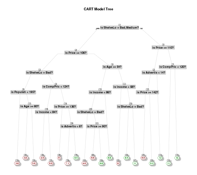
Finally the following shows the CART model tree on the training data.
 1# plot tree
 2cols <- ifelse(mod.reg.caret$frame$yval > 8,"green4","darkred") # green if high
 3prp(mod.reg.caret
 4    ,main="CART Model Tree"
 5    #,extra=106           # display prob of survival and percent of obs
 6    ,nn=TRUE             # display the node numbers
 7    ,fallen.leaves=TRUE  # put the leaves on the bottom of the page
 8    ,branch=.5           # change angle of branch lines
 9    ,faclen=0            # do not abbreviate factor levels
10    ,trace=1             # print the automatically calculated cex
11    ,shadow.col="gray"   # shadows under the leaves
12    ,branch.lty=3        # draw branches using dotted lines
13    ,split.cex=1.2       # make the split text larger than the node text
14    ,split.prefix="is "  # put "is " before split text
15    ,split.suffix="?"    # put "?" after split text
16    ,col=cols, border.col=cols   # green if survived
17    ,split.box.col="lightgray"   # lightgray split boxes (default is white)
18    ,split.border.col="darkgray" # darkgray border on split boxes
19    ,split.round=.5)
## cex 0.65 xlim c(0, 1) ylim c(0, 1)
Comments