While the last three articles illustrated the CART model for both classification (with equal/unequal costs) and regression tasks, this article is rather technical as it compares three packages: rpart, caret and mlr. For those who are not familiar with the last two packages, they are wrappers (or frameworks) that implement a range of models (or algorithms) in a unified way. They are useful because inconsistent API could be a drawback of R (like other open source tools) and it would be quite beneficial if there is a way to implement different models in a standardized way. In line with the earlier articles, the Carseats data is used for a classification task.
Before getting started, I should admit the names are not defined effectively. I hope the below list may be helpful to follow the script.
- package: rpt - rpart, crt - caret, mlr - mlr
- model fitting: ftd - fit on training data, ptd - fit on test data
- parameter selection
- bst - best cp by 1-SE rule (recommended by rpart)
- lst - best cp by highest accuracy (caret) or lowest mmce (mlr)
- cost: eq - equal cost, uq - unequal cost (uq case not added in this article)
- etc: cp - complexity parameter, mmce - mean misclassification error, acc - Accuracy (caret), cm - confusion matrix
Also the data is randomly split into trainData and testData. In practice, the latter is not observed and it is used here for evaludation.
Let’s get started.
The following packages are used.
1library(reshape2)
2library(plyr)
3library(dplyr)
4library(ggplot2)
5library(rpart)
6library(caret)
7library(mlr)
The Sales column is converted into a binary variables.
1## data
2require(ISLR)
3data(Carseats)
4Carseats = Carseats %>%
5  mutate(High=factor(ifelse(Sales<=8,"No","High"),labels=c("High","No")))
6data = subset(Carseats, select=c(-Sales))
Balanced splitting of data can be performed in either of the packages as shown below.
 1## split data
 2# caret
 3set.seed(1237)
 4trainIndex = createDataPartition(Carseats$High, p=0.8, list=FALSE, times=1)
 5trainData.caret = data[trainIndex,]
 6testData.caret = data[-trainIndex,]
 7
 8# mlr
 9set.seed(1237)
10split.desc = makeResampleDesc(method="Holdout", stratify=TRUE, split=0.8)
11split.task = makeClassifTask(data=data,target="High")
12resampleIns = makeResampleInstance(desc=split.desc, task=split.task)
13trainData.mlr = data[resampleIns$train.inds[[1]],]
14testData.mlr = data[-resampleIns$train.inds[[1]],]
15
16# response summaries
17train.res.caret = with(trainData.caret,rbind(table(High),table(High)/length(High)))
18train.res.caret
##            High         No
## [1,] 132.000000 189.000000
## [2,]   0.411215   0.588785
1train.res.mlr = with(trainData.mlr,rbind(table(High),table(High)/length(High)))
2train.res.mlr
##             High          No
## [1,] 131.0000000 188.0000000
## [2,]   0.4106583   0.5893417
1test.res.caret = with(testData.caret,rbind(table(High),table(High)/length(High)))
2test.res.caret
##            High         No
## [1,] 32.0000000 47.0000000
## [2,]  0.4050633  0.5949367
1test.res.mlr = with(testData.mlr,rbind(table(High),table(High)/length(High)))
2test.res.mlr
##            High         No
## [1,] 33.0000000 48.0000000
## [2,]  0.4074074  0.5925926
Same to the previous articles, the split by the caret package is taken.
1# data from caret is taken in line with previous articles
2trainData = trainData.caret
3testData = testData.caret
Note that two custom functions are used: bestParam() and updateCM(). The former searches the cp values by the 1-SE rule (bst) and at the lowest xerror (lst) from the cp table of a rpart object. The latter produces a confusion matrix with model and use error, added to the last column and row respectively. Their sources can be seen here.
1source("src/mlUtils.R")
At first, the model is fit using the rpart package and bst and lst cp values are obtained.
1### rpart
2## train on training data
3set.seed(12357)
4mod.rpt.eq = rpart(High ~ ., data=trainData, control=rpart.control(cp=0))
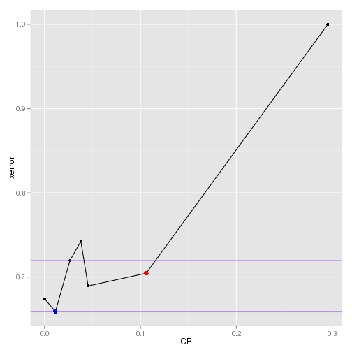
5mod.rpt.eq.par = bestParam(mod.rpt.eq$cptable,"CP","xerror","xstd")
6mod.rpt.eq.par
##            lowest       best
## param  0.01136364 0.10606061
## error  0.65909091 0.70454545
## errStd 0.06033108 0.06157189
The selected cp values can be check graphically below.
 1# plot xerror vs cp
 2df = as.data.frame(mod.rpt.eq$cptable)
 3best = mod.rpt.eq.par
 4ubound = ifelse(best[2,1]+best[3,1]>max(df$xerror),max(df$xerror),best[2,1]+best[3,1])
 5lbound = ifelse(best[2,1]-best[3,1]<min(df$xerror),min(df$xerror),best[2,1]-best[3,1])
 6
 7ggplot(data=df[1:nrow(df),], aes(x=CP,y=xerror)) +
 8  geom_line() + geom_point() +
 9  geom_abline(intercept=ubound,slope=0, color="purple") +
10  geom_abline(intercept=lbound,slope=0, color="purple") +
11  geom_point(aes(x=best[1,2],y=best[2,2]),color="red",size=3) +
12  geom_point(aes(x=best[1,1],y=best[2,1]),color="blue",size=3)
The original tree is pruned with the 2 cp values, resulting in 2 separate trees, and they are fit on the training data.
 1## performance on train data
 2mod.rpt.eq.lst.cp = mod.rpt.eq.par[1,1]
 3mod.rpt.eq.bst.cp = mod.rpt.eq.par[1,2]
 4# prune
 5mod.rpt.eq.lst = prune(mod.rpt.eq, cp=mod.rpt.eq.lst.cp)
 6mod.rpt.eq.bst = prune(mod.rpt.eq, cp=mod.rpt.eq.bst.cp)
 7
 8# fit to train data
 9mod.rpt.eq.lst.ftd = predict(mod.rpt.eq.lst, type="class")
10mod.rpt.eq.bst.ftd = predict(mod.rpt.eq.bst, type="class")
Details of the fitting is kept in a list (mmce).
- pkg: package name
- isTest: fit on test data?
- isBest: cp by 1-SE rule?
- isEq: equal cost?
- cp: cp value used
- mmce: mean misclassification error
 1# fit to train data
 2mod.rpt.eq.lst.ftd = predict(mod.rpt.eq.lst, type="class")
 3mod.rpt.eq.bst.ftd = predict(mod.rpt.eq.bst, type="class")
 4
 5# confusion matrix
 6mod.rpt.eq.lst.ftd.cm = table(actual=trainData$High,fitted=mod.rpt.eq.lst.ftd)
 7mod.rpt.eq.lst.ftd.cm = updateCM(mod.rpt.eq.lst.ftd.cm, type="Fitted")
 8
 9mod.rpt.eq.bst.ftd.cm = table(actual=trainData$High,fitted=mod.rpt.eq.bst.ftd)
10mod.rpt.eq.bst.ftd.cm = updateCM(mod.rpt.eq.bst.ftd.cm, type="Fitted")
11
12# misclassification error
13mod.rpt.eq.lst.ftd.mmce = list(pkg="rpart",isTest=FALSE,isBest=FALSE,isEq=TRUE
14                               ,cp=round(mod.rpt.eq.lst.cp,4)
15                               ,mmce=mod.rpt.eq.lst.ftd.cm[3,3])
16mmce = list(unlist(mod.rpt.eq.lst.ftd.mmce))
17
18mod.rpt.eq.bst.ftd.mmce = list(pkg="rpart",isTest=FALSE,isBest=TRUE,isEq=TRUE
19                               ,cp=round(mod.rpt.eq.bst.cp,4)
20                              ,mmce=mod.rpt.eq.bst.ftd.cm[3,3])
21mmce[[length(mmce)+1]] = unlist(mod.rpt.eq.bst.ftd.mmce)
22
23ldply(mmce)
##     pkg isTest isBest isEq     cp mmce
## 1 rpart  FALSE  FALSE TRUE 0.0114 0.16
## 2 rpart  FALSE   TRUE TRUE 0.1061 0.29
The pruned trees are fit into the test data and the same details are added to the list (mmce).
 1## performance of test data
 2# fit to test data
 3mod.rpt.eq.lst.ptd = predict(mod.rpt.eq.lst, newdata=testData, type="class")
 4mod.rpt.eq.bst.ptd = predict(mod.rpt.eq.bst, newdata=testData, type="class")
 5
 6# confusion matrix
 7mod.rpt.eq.lst.ptd.cm = table(actual=testData$High, fitted=mod.rpt.eq.lst.ptd)
 8mod.rpt.eq.lst.ptd.cm = updateCM(mod.rpt.eq.lst.ptd.cm)
 9
10mod.rpt.eq.bst.ptd.cm = table(actual=testData$High, fitted=mod.rpt.eq.bst.ptd)
11mod.rpt.eq.bst.ptd.cm = updateCM(mod.rpt.eq.bst.ptd.cm)
12
13# misclassification error
14mod.rpt.eq.lst.ptd.mmce = list(pkg="rpart",isTest=TRUE,isBest=FALSE,isEq=TRUE
15                               ,cp=round(mod.rpt.eq.lst.cp,4)
16                               ,mmce=mod.rpt.eq.lst.ptd.cm[3,3])
17mmce[[length(mmce)+1]] = unlist(mod.rpt.eq.lst.ptd.mmce)
18
19mod.rpt.eq.bst.ptd.mmce = list(pkg="rpart",isTest=TRUE,isBest=TRUE,isEq=TRUE
20                               ,cp=round(mod.rpt.eq.bst.cp,4)
21                              ,mmce=mod.rpt.eq.bst.ptd.cm[3,3])
22mmce[[length(mmce)+1]] = unlist(mod.rpt.eq.bst.ptd.mmce)
23
24ldply(mmce)
##     pkg isTest isBest isEq     cp mmce
## 1 rpart  FALSE  FALSE TRUE 0.0114 0.16
## 2 rpart  FALSE   TRUE TRUE 0.1061 0.29
## 3 rpart   TRUE  FALSE TRUE 0.0114 0.19
## 4 rpart   TRUE   TRUE TRUE 0.1061  0.3
Secondly the caret package is employed to implement the CART model.
1### caret
2## train on training data
3trControl = trainControl(method="repeatedcv", number=10, repeats=5)
4set.seed(12357)
5mod.crt.eq = caret::train(High ~ .
6                          ,data=trainData
7                          ,method="rpart"
8                          ,tuneLength=20
9                          ,trControl=trControl)
Note that the caret package select the best cp value that corresponds to the lowest Accuracy. Therefore the best cp by this package is labeled as lst to be consistent with the rpart package. And the bst cp is selected by the 1-SE rule. Note that, as the standard error of Accuracy is relatively wide, an adjustment is maded to select the best cp value and it can be checked in the graph below.
 1# lowest CP
 2# caret: maximum accuracy, rpart: 1-SE
 3# according to rpart, caret's best is lowest
 4df = mod.crt.eq$results
 5mod.crt.eq.lst.cp = mod.crt.eq$bestTune$cp
 6mod.crt.eq.lst.acc = subset(df,cp==mod.crt.eq.lst.cp)[[2]]
 7
 8# best cp by 1-SE rule - values are adjusted from graph
 9mod.crt.eq.bst.cp = df[17,1]
10mod.crt.eq.bst.acc = df[17,2]
 1# CP by 1-SE rule
 2maxAcc = subset(df,Accuracy==max(Accuracy))[[2]]
 3stdAtMaxAcc = subset(df,subset=Accuracy==max(Accuracy))[[4]]
 4# max cp within 1 SE
 5maxCP = subset(df,Accuracy>=maxAcc-stdAtMaxAcc)[nrow(subset(df,Accuracy>=maxAcc-stdAtMaxAcc)),][[1]]
 6accAtMaxCP = subset(df,cp==maxCP)[[2]]
 7
 8# plot Accuracy vs cp
 9ubound = ifelse(maxAcc+stdAtMaxAcc>max(df$Accuracy),max(df$Accuracy),maxAcc+stdAtMaxAcc)
10lbound = ifelse(maxAcc-stdAtMaxAcc<min(df$Accuracy),min(df$Accuracy),maxAcc-stdAtMaxAcc)
11
12ggplot(data=df[1:nrow(df),], aes(x=cp,y=Accuracy)) +
13  geom_line() + geom_point() +
14  geom_abline(intercept=ubound,slope=0, color="purple") +
15  geom_abline(intercept=lbound,slope=0, color="purple") +
16  geom_point(aes(x=mod.crt.eq.bst.cp,y=mod.crt.eq.bst.acc),color="red",size=3) +
17  geom_point(aes(x=mod.crt.eq.lst.cp,y=mod.crt.eq.lst.acc),color="blue",size=3)
![]()
Similar to above, 2 trees with the respective cp values are fit into the train and test data and the details are kept in mmce. Below is the update by fitting from the train data.
 1## performance on train data
 2# refit from rpart for best cp - cp by 1-SE not fitted by caret
 3# note no cross-validation necessary - xval=0 (default: xval=10)
 4set.seed(12357)
 5mod.crt.eq.bst = rpart(High ~ ., data=trainData, control=rpart.control(xval=0,cp=mod.crt.eq.bst.cp))
 6
 7# fit to train data - lowest from caret, best (1-SE) from rpart
 8mod.crt.eq.lst.ftd = predict(mod.crt.eq,newdata=trainData)
 9mod.crt.eq.bst.ftd = predict(mod.crt.eq.bst, type="class")
10
11# confusion matrix
12mod.crt.eq.lst.ftd.cm = table(actual=trainData$High,fitted=mod.crt.eq.lst.ftd)
13mod.crt.eq.lst.ftd.cm = updateCM(mod.crt.eq.lst.ftd.cm, type="Fitted")
14
15mod.crt.eq.bst.ftd.cm = table(actual=trainData$High,fitted=mod.crt.eq.bst.ftd)
16mod.crt.eq.bst.ftd.cm = updateCM(mod.crt.eq.bst.ftd.cm, type="Fitted")
17
18# misclassification error
19mod.crt.eq.lst.ftd.mmce = list(pkg="caret",isTest=FALSE,isBest=FALSE,isEq=TRUE
20                               ,cp=round(mod.crt.eq.lst.cp,4)
21                               ,mmce=mod.crt.eq.lst.ftd.cm[3,3])
22mmce[[length(mmce)+1]] = unlist(mod.crt.eq.lst.ftd.mmce)
23
24mod.crt.eq.bst.ftd.mmce = list(pkg="caret",isTest=FALSE,isBest=TRUE,isEq=TRUE
25                               ,cp=round(mod.crt.eq.bst.cp,4)
26                               ,mmce=mod.crt.eq.bst.ftd.cm[3,3])
27mmce[[length(mmce)+1]] = unlist(mod.crt.eq.bst.ftd.mmce)
Below is the update by fitting from the test data. The updated fitting details can be checked.
 1## performance of test data
 2# fit to test data - lowest from caret, best (1-SE) from rpart
 3mod.crt.eq.lst.ptd = predict(mod.crt.eq,newdata=testData)
 4mod.crt.eq.bst.ptd = predict(mod.crt.eq.bst, newdata=testData)
 5
 6# confusion matrix
 7mod.crt.eq.lst.ptd.cm = table(actual=testData$High, fitted=mod.rpt.eq.lst.ptd)
 8mod.crt.eq.lst.ptd.cm = updateCM(mod.crt.eq.lst.ptd.cm)
 9
10mod.crt.eq.bst.ptd.cm = table(actual=testData$High, fitted=mod.rpt.eq.bst.ptd)
11mod.crt.eq.bst.ptd.cm = updateCM(mod.crt.eq.bst.ptd.cm)
12
13# misclassification error
14mod.crt.eq.lst.ptd.mmce = list(pkg="caret",isTest=TRUE,isBest=FALSE,isEq=TRUE
15                               ,cp=round(mod.crt.eq.lst.cp,4)
16                               ,mmce=mod.crt.eq.lst.ptd.cm[3,3])
17mmce[[length(mmce)+1]] = unlist(mod.crt.eq.lst.ptd.mmce)
18
19mod.crt.eq.bst.ptd.mmce = list(pkg="caret",isTest=TRUE,isBest=TRUE,isEq=TRUE
20                               ,cp=round(mod.crt.eq.bst.cp,4)
21                               ,mmce=mod.crt.eq.bst.ptd.cm[3,3])
22mmce[[length(mmce)+1]] = unlist(mod.crt.eq.bst.ptd.mmce)
23
24ldply(mmce)
##     pkg isTest isBest isEq     cp mmce
## 1 rpart  FALSE  FALSE TRUE 0.0114 0.16
## 2 rpart  FALSE   TRUE TRUE 0.1061 0.29
## 3 rpart   TRUE  FALSE TRUE 0.0114 0.19
## 4 rpart   TRUE   TRUE TRUE 0.1061  0.3
## 5 caret  FALSE  FALSE TRUE 0.0156 0.16
## 6 caret  FALSE   TRUE TRUE 0.2488 0.29
## 7 caret   TRUE  FALSE TRUE 0.0156 0.19
## 8 caret   TRUE   TRUE TRUE 0.2488  0.3
Finally the mlr package is employed.
At first, a taks and learner are set up.
1### mlr
2## task and learner
3tsk.mlr.eq = makeClassifTask(data=trainData,target="High")
4lrn.mlr.eq = makeLearner("classif.rpart",par.vals=list(cp=0))
Then a grid of cp values is generated followed by tuning the parameter. Note that, as the tuning optimization path does not include a standard-error-like variable, only the best cp values are taken into consideration.
 1## tune parameter
 2cpGrid = function(index) {
 3  start=0
 4  end=0.3
 5  len=20
 6  inc = (end-start)/len
 7  grid = c(start)
 8  while(start < end) {
 9    start = start + inc
10    grid = c(grid,start)
11  }
12  grid[index]
13}
14# create tune control grid
15ps.mlr.eq = makeParamSet(
16    makeNumericParam("cp",lower=1,upper=20,trafo=cpGrid)
17  )
18ctrl.mlr.eq = makeTuneControlGrid(resolution=c(cp=(20)))
19
20# tune cp
21rdesc.mlr.eq = makeResampleDesc("RepCV",reps=5,folds=10,stratify=TRUE)
22set.seed(12357)
23tune.mlr.eq = tuneParams(learner=lrn.mlr.eq
24                         ,task=tsk.mlr.eq
25                         ,resampling=rdesc.mlr.eq
26                         ,par.set=ps.mlr.eq
27                         ,control=ctrl.mlr.eq)
28# tuned cp
29tune.mlr.eq$x
## $cp
## [1] 0.015
1# optimization path
2# no standard error like values, only best cp is considered
3path.mlr.eq = as.data.frame(tune.mlr.eq$opt.path)
4path.mlr.eq = transform(path.mlr.eq,cp=cpGrid(cp))
5head(path.mlr.eq,3)
##      cp mmce.test.mean dob eol error.message exec.time
## 1 0.000      0.2623790   1  NA          <NA>     0.948
## 2 0.015      0.2555407   2  NA          <NA>     0.944
## 3 0.030      0.2629069   3  NA          <NA>     0.945
Using the best cp value, the learner is updated followed by training the model.
1# obtain fitted and predicted responses
2# update cp
3lrn.mlr.eq.bst = setHyperPars(lrn.mlr.eq, par.vals=tune.mlr.eq$x)
4
5# train model
6trn.mlr.eq.bst = train(lrn.mlr.eq.bst, tsk.mlr.eq)
Then the model is fit into the train and test data and the fitting details are updated in mmce. The overall fitting results can be checked below.
 1# fitted responses
 2mod.mlr.eq.bst.ftd = predict(trn.mlr.eq.bst, tsk.mlr.eq)$data
 3mod.mlr.eq.bst.ptd = predict(trn.mlr.eq.bst, newdata=testData)$data
 4
 5# confusion matrix
 6mod.mlr.eq.bst.ftd.cm = table(actual=mod.mlr.eq.bst.ftd$truth, fitted=mod.mlr.eq.bst.ftd$response)
 7mod.mlr.eq.bst.ftd.cm = updateCM(mod.mlr.eq.bst.ftd.cm)
 8
 9mod.mlr.eq.bst.ptd.cm = table(actual=mod.mlr.eq.bst.ptd$truth, fitted=mod.mlr.eq.bst.ptd$response)
10mod.mlr.eq.bst.ptd.cm = updateCM(mod.mlr.eq.bst.ptd.cm)
11
12# misclassification error
13mod.mlr.eq.bst.ftd.mmce = list(pkg="mlr",isTest=FALSE,isBest=FALSE,isEq=TRUE
14                               ,cp=round(tune.mlr.eq$x[[1]],4)
15                               ,mmce=mod.mlr.eq.bst.ftd.cm[3,3])
16mmce[[length(mmce)+1]] = unlist(mod.mlr.eq.bst.ftd.mmce)
17
18mod.mlr.eq.bst.ptd.mmce = list(pkg="mlr",isTest=TRUE,isBest=FALSE,isEq=TRUE
19                               ,cp=round(tune.mlr.eq$x[[1]],4)
20                               ,mmce=mod.mlr.eq.bst.ptd.cm[3,3])
21mmce[[length(mmce)+1]] = unlist(mod.mlr.eq.bst.ptd.mmce)
22
23ldply(mmce)
##      pkg isTest isBest isEq     cp mmce
## 1  rpart  FALSE  FALSE TRUE 0.0114 0.16
## 2  rpart  FALSE   TRUE TRUE 0.1061 0.29
## 3  rpart   TRUE  FALSE TRUE 0.0114 0.19
## 4  rpart   TRUE   TRUE TRUE 0.1061  0.3
## 5  caret  FALSE  FALSE TRUE 0.0156 0.16
## 6  caret  FALSE   TRUE TRUE 0.2488 0.29
## 7  caret   TRUE  FALSE TRUE 0.0156 0.19
## 8  caret   TRUE   TRUE TRUE 0.2488  0.3
## 9    mlr  FALSE  FALSE TRUE  0.015 0.16
## 10   mlr   TRUE  FALSE TRUE  0.015 0.19
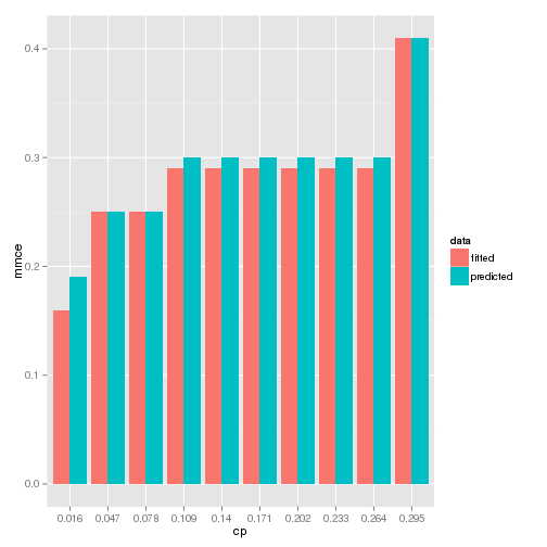
It is shown that the mmce values are identical and it seems to be because the model is quite stable with respect to cp. It can be checked in the following graph.
 1# mmce vs cp
 2ftd.mmce = c()
 3ptd.mmce = c()
 4cps = mod.crt.eq$results[[1]]
 5for(i in 1:length(cps)) {
 6  if(i %% 2 == 0) {
 7    set.seed(12357)
 8    mod = rpart(High ~ ., data=trainData, control=rpart.control(cp=cps[i]))
 9    ftd = predict(mod,type="class")
10    ptd = predict(mod,newdata=testData,type="class")
11    ftd.mmce = c(ftd.mmce,updateCM(table(trainData$High,ftd))[3,3])
12    ptd.mmce = c(ptd.mmce,updateCM(table(testData$High,ptd))[3,3])
13  }
14}
15mmce.crt = data.frame(cp=as.factor(round(cps[seq(2,length(cps),2)],3))
16                      ,fitted=ftd.mmce
17                      ,predicted=ptd.mmce)
18mmce.crt = melt(mmce.crt,id=c("cp"),variable.name="data",value.name="mmce")
19ggplot(data=mmce.crt,aes(x=cp,y=mmce,fill=data)) +
20  geom_bar(stat="identity", position=position_dodge())
It may not be convicing to use a wrapper by this article about a single model. For example, however, if there are multiple models with a variety of tuning parameters to compare, the benefit of having one can be considerable. In the following articles, a similar approach would be taken, which is comparing individual packages to the wrappers.
Comments