This article evaluates a single regression tree’s performance by comparing to bagged trees’ individual oob/test errors, cumulative oob/test errors and variable importance measures.
Before getting started, note that the source of the classes can be found in this gist and, together with the relevant packages (see tags), it requires a utility function (bestParam()) that can be found here.
Data is split as usual.
 1## data
 2require(ISLR)
 3data(Carseats)
 4require(dplyr)
 5Carseats = Carseats %>%
 6  mutate(High=factor(ifelse(Sales<=8,"No","High"),labels=c("High","No")))
 7data.cl = subset(Carseats, select=c(-Sales))
 8data.rg = subset(Carseats, select=c(-High))
 9
10# split data
11require(caret)
12set.seed(1237)
13trainIndex = createDataPartition(Carseats$High, p=0.8, list=FALSE, times=1)
14trainData.rg = data.rg[trainIndex,]
15testData.rg = data.rg[-trainIndex,]
Both the single and bagged regression trees are fit. For bagging, 2000 trees are generated.
1## run rpartDT
2# import constructors
3source("src/cart.R")
4set.seed(12357)
5rg = cartDT(trainData.rg, testData.rg, "Sales ~ .", ntree=2000)
The summary of the cp values of the bagged trees are shown below, followed by the single tree’s cp value at the least xerror.
1## cp values
2# cart
3rg$rpt$cp[1,][[1]]
## [1] 0.004852267
1# bagging
2summary(t(rg$boot.cp)[,2])
##     Min.  1st Qu.   Median     Mean  3rd Qu.     Max.
## 0.000000 0.000000 0.000000 0.001430 0.002568 0.018640
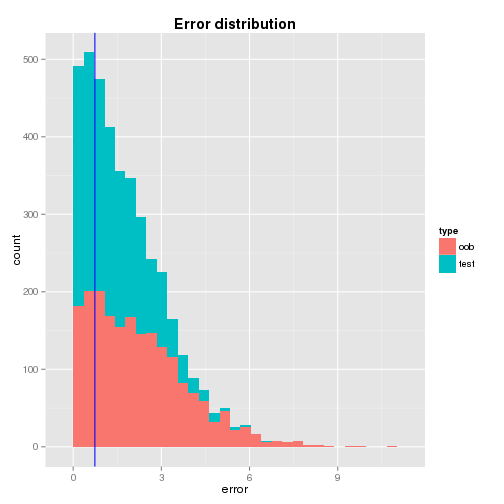
Individual Error
From the distributions of the oob and test errors, it is found that
- the single tree’s test error is not far away from the means of the bagged trees’ oob and test errors - it is only 0.92 and 0.65 standard deviation away repectively and
- the distributions are dense in the left hand side where the single tree’s test error locates so that it may be considered that the test error is a likely value.
1## individual errors
2# cart test error
3crt.err = rg$rpt$test.lst$error$error
4crt.err
## [1] 0.737656
1# bagging error at least xerror - se to see 1-SE rule
2ind.oob.err = data.frame(type="oob",error=unlist(rg$ind.oob.lst.err))
3ind.tst.err = data.frame(type="test",error=unlist(rg$ind.tst.lst.err))
4ind.err = rbind(ind.oob.err,ind.tst.err)
5ind.err.summary = as.data.frame(rbind(summary(ind.err$error[ind.err$type=="oob"])
6                                      ,summary(ind.err$error[ind.err$type=="test"])))
7rownames(ind.err.summary) <- c("oob","test")
8ind.err.summary
##           Min. 1st Qu. Median  Mean 3rd Qu.   Max.
## oob  0.0053970  0.9026  1.972 2.247   3.207 10.670
## test 0.0005156  0.5734  1.217 1.442   2.107  6.738
A graphical illustration of the error distributions and the location of the single tree’s test error are shown below.
1# plot error distributions
2ggplot(ind.err, aes(x=error,fill=type)) +
3  geom_histogram() + geom_vline(xintercept=crt.err, color="blue") +
4  ggtitle("Error distribution") + theme(plot.title=element_text(face="bold"))
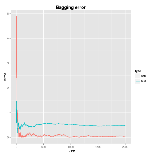
Cumulative Error
The plots of cumulative oob and test errors are shown below and both the errors seem to settle around 1000th tree. The oob and test errors at the 1000th tree are 0.018 and 0.512 respectively. Compared to the single tree’s test error of 0.738, the bagged trees deliveres imporved results.
 1bgg.oob.err = data.frame(type="oob"
 2                         ,ntree=1:length(rg$cum.oob.lst.err)
 3                         ,error=unlist(rg$cum.oob.lst.err))
 4bgg.tst.err = data.frame(type="test"
 5                         ,ntree=1:length(rg$cum.tst.lst.err)
 6                         ,error=unlist(rg$cum.tst.lst.err))
 7bgg.err = rbind(bgg.oob.err,bgg.tst.err)
 8# plot bagging errors
 9ggplot(data=bgg.err,aes(x=ntree,y=error,colour=type)) +
10  geom_line() + geom_abline(intercept=crt.err,slope=0,color="blue") +
11  ggtitle("Bagging error") + theme(plot.title=element_text(face="bold"))
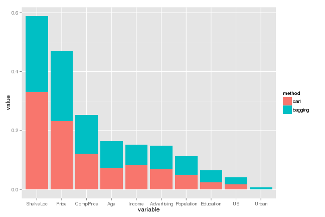
Variable Importance
While ShelveLoc and Price are shown to be the two most important variables, both the single and bagged trees show similar variable importance profiles. For evaluating a single tree, this would be a positive result as it could show that the splits of the single tree is reinforced to be valid by the bagged trees.
For prediction, however, there may be some room for improvement as the bagged trees might be correlated to some extent, especially due to the existence of the two important variables. For example, if earlier splits are determined by these predictors, there are not enough chances for the remaining predictors and it is not easy to identify local systematic patterns.
 1# cart
 2cart.varImp = data.frame(method="cart"
 3                         ,variable=names(rg$rpt$mod$variable.importance)
 4                         ,value=rg$rpt$mod$variable.importance/sum(rg$rpt$mod$variable.importance)
 5                         ,row.names=NULL)
 6# bagging
 7ntree = 1000
 8bgg.varImp = data.frame(method="bagging"
 9                        ,variable=rownames(rg$cum.varImp.lst)
10                        ,value=rg$cum.varImp.lst[,ntree])
11# plot variable importance measure
12rg.varImp = rbind(cart.varImp,bgg.varImp)
13rg.varImp$variable = reorder(rg.varImp$variable, 1/rg.varImp$value)
14ggplot(data=rg.varImp,aes(x=variable,y=value,fill=method)) + geom_bar(stat="identity")
In this article, a single regression tree is evaluated by bagged trees. Comparing to individual oob/test errors, the single tree’s test error seems to be a likely value. Also, while bagged trees improve prediction performance, the single tree may not be a bad choice especially if more focus is on interpretation. Despite the performance improvement of the bagged trees, there seems to be a chance for additional improvement and the right direction of subsequence articles would be looking into it.
Comments