A regression tree is evaluated using bagged trees in the previous article. In this article, the response variable of the same data set is converted into a binary factor variable and a classification tree is evaluated by comparing to bagged trees’ individual oob/test errors, cumulative oob/test errors and variable importance measures.
Before getting started, note that the source of the classes can be found in this gist and, together with the relevant packages (see tags), it requires a utility function (bestParam()) that can be found here.
Data is split as usual.
 1## data
 2require(ISLR)
 3data(Carseats)
 4require(dplyr)
 5Carseats = Carseats %>%
 6  mutate(High=factor(ifelse(Sales<=8,"No","High"),labels=c("High","No")))
 7data.cl = subset(Carseats, select=c(-Sales))
 8data.rg = subset(Carseats, select=c(-High))
 9
10# split data
11require(caret)
12set.seed(1237)
13trainIndex = createDataPartition(Carseats$High, p=0.8, list=FALSE, times=1)
14trainData.cl = data.cl[trainIndex,]
15testData.cl = data.cl[-trainIndex,]
Both the single and bagged classification trees are fit. For bagging, 500 trees are generated - as shown below, the cumulative test error settles well before this number of trees but this is not the case for the cumulative oob error. The number of the trees is just set rather than tuned in this article.
1## run rpartDT
2# import constructors
3source("src/cart.R")
4set.seed(12357)
5cl = cartDT(trainData.cl, testData.cl, "High ~ .", ntree=500)
The summary of the cp values of the bagged trees are shown below, followed by the single tree’s cp value at the least xerror.
1## cp values
2# cart
3cl$rpt$cp[1,][[1]]
## [1] 0.01136364
1# bagging
2summary(t(cl$boot.cp)[,2])
##     Min.  1st Qu.   Median     Mean  3rd Qu.     Max.
## 0.000000 0.000000 0.002407 0.007940 0.014930 0.048950
Individual Error
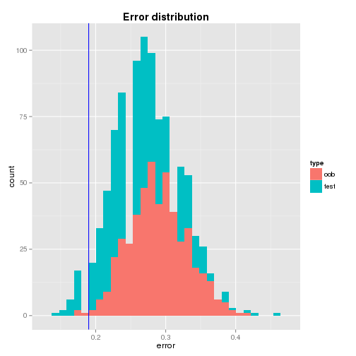
From the distributions of the oob and test errors, it is found that
- the distributions are roughly bell-shaped where the centers are closer to 0.3 - interestingly the mean of the oob error (0.29) is higher than that of the test error (0.26) while their standard deviations are not that much different,
- the single tree’s test error is quite away from the means of the bagged trees’ oob and test errors - it is 2.38 and 1.43 standard deviation away repectively and
- the test error of the single tree (0.19) seems to be quite optimistic.
1## individual errors
2# cart test error
3crt.err = cl$rpt$test.lst$error$error
4crt.err
## [1] 0.19
1# bagging error at least xerror - se to see 1-SE rule
2ind.oob.err = data.frame(type="oob",error=unlist(cl$ind.oob.lst.err))
3ind.tst.err = data.frame(type="test",error=unlist(cl$ind.tst.lst.err))
4ind.err = rbind(ind.oob.err,ind.tst.err)
5ind.err.summary = as.data.frame(rbind(summary(ind.err$error[ind.err$type=="oob"])
6                                      ,summary(ind.err$error[ind.err$type=="test"])))
7rownames(ind.err.summary) <- c("oob","test")
8ind.err.summary
##        Min. 1st Qu. Median   Mean 3rd Qu.   Max.
## oob  0.1695  0.2605 0.2881 0.2890  0.3162 0.4182
## test 0.1392  0.2278 0.2532 0.2593  0.2911 0.4557
A graphical illustration of the error distributions and the location of the single tree’s test error are shown below.
1# plot error distribution
2ggplot(ind.err, aes(x=error,fill=type)) +
3  geom_histogram() + geom_vline(xintercept=crt.err, color="blue") +
4  ggtitle("Error distribution") + theme(plot.title=element_text(face="bold"))
Cumulative Error
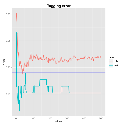
The plots of cumulative oob and test errors are shown below. It is found that, while the cumulative test error (0.152) settles just after the 300th tree and it is lower than the single tree’s test error (0.19), the cumulative oob error fluctuates and it is higher than that of the single tree - the error at the 500th tree is 0.218 (the oob error doesn’t settle even a higher number of trees are tried).
It would be understood as following.
- Hastie et al.(2008) demonstrates that an aggregate estimator tends to decrease mean-squared error as averaging can lower variance and leaves bias unchanged. However, as bias and variance are non-additive, it does not hold for classification under 0-1 loss and an aggregate estimator’s performance depends on how good the classifer is.
- Also, compared to the cumulative test error, the single tree seems to overfit the train data so that its prediction power is impared.
- According to the above demonstration and comparison to the cumulative test error, the quality of the CART model as a classifier might be questionable for this data set.
 1bgg.oob.err = data.frame(type="oob"
 2                         ,ntree=1:length(cl$cum.oob.lst.err)
 3                         ,error=unlist(cl$cum.oob.lst.err))
 4bgg.tst.err = data.frame(type="test"
 5                         ,ntree=1:length(cl$cum.tst.lst.err)
 6                         ,error=unlist(cl$cum.tst.lst.err))
 7bgg.err = rbind(bgg.oob.err,bgg.tst.err)
 8
 9# plot bagging errors
10ggplot(data=bgg.err,aes(x=ntree,y=error,colour=type)) +
11  geom_line() + geom_abline(intercept=crt.err,slope=0,color="blue") +
12  ggtitle("Bagging error") + theme(plot.title=element_text(face="bold"))
Variable Importance
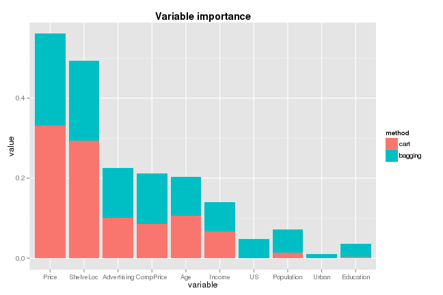
Like the regression task, Price and ShelveLoc are shown to be the two most important variables although their ranks are reversed. In the single tree, these variables are more valued than bagging and the bottom 4 variables are measured having little value - even US and Urban are not employed to reduce impurity.
Difference in composition of the variable importance measures and concentration to the top 2 variables seems to bring more questions with regard to its effectiveness as a classifier for this data set.
 1# cart
 2cart.varImp = data.frame(method="cart"
 3                         ,variable=names(cl$rpt$mod$variable.importance)
 4                         ,value=cl$rpt$mod$variable.importance/sum(cl$rpt$mod$variable.importance)
 5                         ,row.names=NULL)
 6# bagging
 7ntree = length(cl$cum.varImp.lst)
 8bgg.varImp = data.frame(method="bagging"
 9                        ,variable=rownames(cl$cum.varImp.lst)
10                        ,value=cl$cum.varImp.lst[,ntree])
11# plot variable importance measure
12cl.varImp = rbind(cart.varImp,bgg.varImp)
13cl.varImp$variable = reorder(cl.varImp$variable, 1/cl.varImp$value)
14ggplot(data=cl.varImp,aes(x=variable,y=value,fill=method)) + geom_bar(stat="identity") +
15  ggtitle("Variable importance") + theme(plot.title=element_text(face="bold"))
In this article, a classification tree is evaluated comparing to bagged trees. In comparison to individual oob/test errors, the single tree’s test error seems to be quite optimistic. Also oob samples doesn’t improve prediction performance as the tree generating process might be dominated by a few predictors. Comparing to the cumulative test error, it seems that the single tree overfits the train data so that its prediction power is not competitive. Although the CART model as a classifier doesn’t seem to be attractive for this data set, it may be a bit early to discard it. What seems to be necessary is to check the cases where the dominant predictors’ impacts are reduced and subsequent articles would head toward that direction.
Comments