Prototyping a Live Product Recommender With Python

Overview

Traditional recommendation systems, like Collaborative Filtering, are widely used but have limitations. They struggle with the cold-start problem (new users have no history) and rely heavily on long-term signals. They also often ignore short-term context such as time of day, device, location, or session intent, and can miss nuances, for example, a user wanting coffee in the morning but pizza at night.

Contextual Multi-Armed Bandits (CMAB) address these gaps through online learning.

As a practical form of reinforcement learning, CMAB balances two goals in real time:

1. Exploitation: Recommending what is known to work.
2. Exploration: Trying less-tested options to discover new favorites.

By conditioning decisions on live context, CMAB adapts instantly to changing user behavior.

Why CMAB?

• Beyond A/B Testing: Instead of finding a single global winner, CMAB enables 1:1 personalization, selecting the best option for this user in this context.
• Real-Time Adaptation: Unlike batch-trained models that quickly become stale, CMAB updates incrementally, making it ideal for news/products recommendation, dynamic pricing, or inventory-aware ranking.

Several CMAB implementations exist, including Vowpal Wabbit and River ML. In this post, we use Mab2Rec for offline policy evaluation and MABWiser to build the live recommender prototype.

Data Streaming Opportunity

CMAB performs well in data streaming environments. Integrated with platforms like Kafka and Flink, it learns directly from event streams, creating a feedback loop that responds to trends and shifts in user intent in sub-seconds.

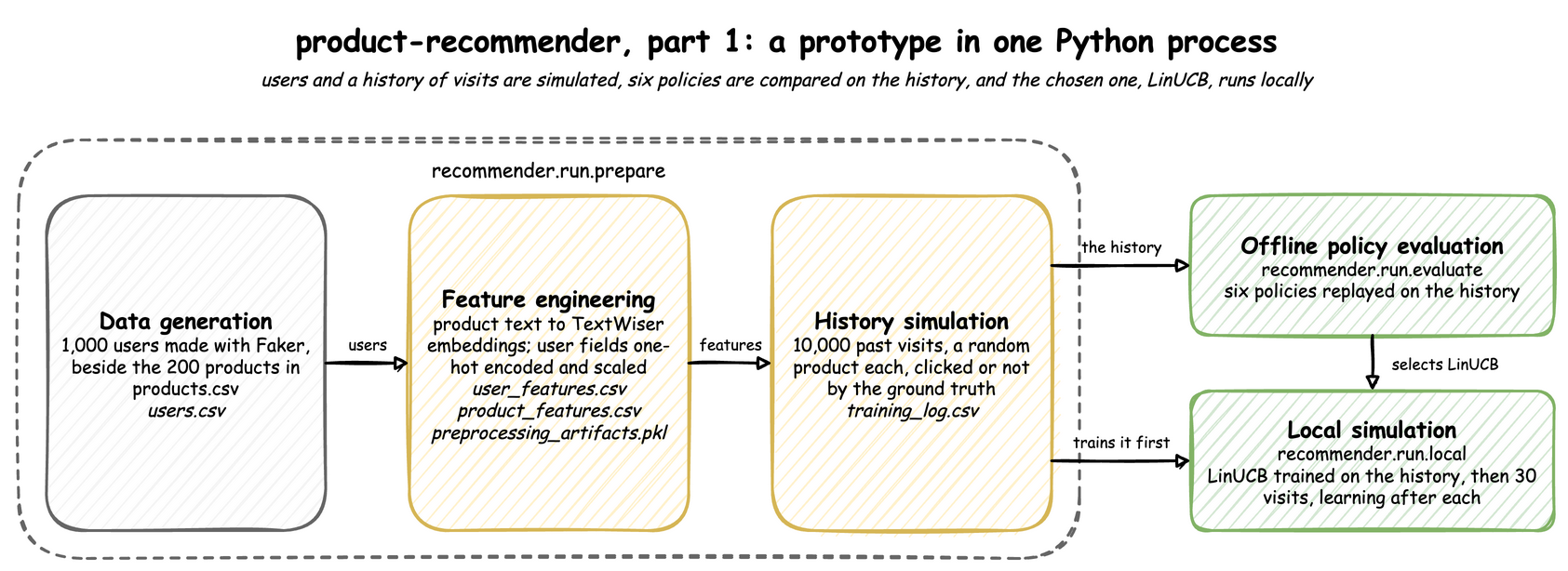
In this series, Part 1 (this post) builds a complete Python prototype to validate the algorithm and simulate user behavior. Part 2 (coming soon) will scale this to a distributed, event-driven architecture.

Tech Stack

We are building this prototype using Python 3.11.

Engineering Note: We explicitly chose Python 3.11 because parts of our stack (specifically mabwiser dependencies) rely on older versions of pandas (< 2.0). On Python 3.12+, installing these dependencies often triggers long compilation times or failures due to missing binary wheels.

We use uv for Python environment management. The core libraries include:

• MABWiser: The engine. It implements the core Contextual Bandit algorithms.
• Mab2Rec: The vehicle. A high-level wrapper that streamlines Recommender System pipelines.
• TextWiser: For converting raw text features into numerical embeddings.
• scikit-learn: For feature scaling and encoding.
• Faker & Pandas: For synthetic data generation and simulation.

The development environment can be constructed as follows:

 1$ git clone https://github.com/jaehyeon-kim/streaming-demos.git
 2$ cd streaming-demos
 3$ uv python install 3.11
 4$ uv venv --python 3.11 venv
 5$ source venv/bin/activate
 6(venv) $ uv pip install -r product-recommender/requirements.txt
 7(venv) $ uv pip list | grep -E "mab|wiser|panda|numpy|scikit|faker"
 8# Using Python 3.11.14 environment at: venv
 9# faker                              40.1.2
10# mab2rec                            1.3.1
11# mabwiser                           2.7.4
12# numpy                              1.26.4
13# pandas                             1.5.3
14# scikit-learn                       1.8.0
15# textwiser                          2.0.2

📂 Source Code for the Post

The source code for this post is available in the product-recommender folder of the streaming-demos GitHub repository.

Data Generation

We first need product and user data to generate the required features.

Products

We utilize a set of 200 raw products, each containing a product ID, name, text description, price, and high-level category.

Here is a list of sample products:

Users

We generate 1,000 Synthetic Users using Faker. Each user is assigned static attributes like Age, Gender, Location, and Traffic Source. These attributes will serve as the “Context” for our Bandit.

Here is a sample of our user base:

Note that street address, postal code, city, state, and country are omitted, as only latitude and longitude are used for feature generation.

Feature Engineering

Bandit algorithms operate on numerical vectors, not raw text. In other words, they cannot interpret "Burger" unless it is converted into numbers. To address this, we developed a transformation pipeline to properly prepare our data:

1. Product Features: We used TextWiser to convert raw product descriptions into vector embeddings. This allows the model to understand that “Burger” and “Sandwich” are semantically closer than “Burger” and “Headphones”. We also applied One-Hot Encoding to categories (Product Category) and MinMax scaling to the price. Finally, we added a binary feature, is_coffee, which is set to 1 for coffee products (e.g., espresso, cappuccino) and 0 otherwise.
2. User Features: Similar to the product features, we applied One-Hot Encoding to categories (Gender and Traffic Source) and MinMax scaling to numerical fields (Age, Latitude, and Longitude).
3. Pipeline Artifacts: We save these transformers as preprocessing_artifacts.pkl. This allows our system to instantly transform any new user/product record into a compatible feature vector during inference.

Sample Processed Product Features:

Notice how the description is now represented by txt_0…txt_9 embeddings.

Sample Processed User Features:

Notice that Age, Latitude and Longitude are normalized between 0 and 1, and categorical fields are binary.

Bandit History Simulation

To evaluate whether our model can truly learn user behavior, we need a controlled Ground Truth, which is an Oracle that determines the likelihood of a simulated user clicking on a recommendation.

Crucially, this Oracle is hidden from the model. The model’s task is to infer these patterns purely from trial and error.

We also inject Dynamic Context features like Time of Day and Day of Week into the user profile at the moment of interaction. These temporal signals create realistic, fluctuating patterns that the model must adapt to.

Simulation Logic

The simulation is implemented as a class GroundTruth, and we define specific rules that govern user behaviour:

• Start from a low base logit (−2.5) to model generally low click probability.
• Rule 1: Morning coffee preference: if the user is browsing in the morning and the item is a coffee product, add a strong positive boost to the score.
• Rule 2: Weekend comfort food: if the session is on a weekend and the item is Pizza or Burgers & Sandwiches, add a moderate positive boost.
• Rule 3: Budget sensitivity: if the user is young (normalized age < 0.25) and the item is expensive (normalized price > 0.8), apply a strong negative penalty.
• Rule 4: Traffic source bias: if the user arrived via Search, add a small intent-based boost.
• Convert the final logit score into a click probability using a sigmoid function, then sample a Bernoulli trial to simulate whether a click occurs.

 1# product-recommender/recsys-engine/src/bandit_simulator.py
 2class GroundTruth:
 3    """
 4    The HIDDEN FORMULA (Ground Truth) for click simulation.
 5    Determines user click behavior based on context and item features.
 6    """
 7
 8    @staticmethod
 9    def calculate_probability(user_ctx: dict, item_ctx: dict) -> float:
10        """
11        Computes the probability that a user clicks an item.
12        Uses logistic regression-style scoring with domain-specific rules.
13        """
14        score = -2.5  # Base logit: starts with a low probability
15
16        # Rule 1: Morning Coffee
17        # Users are more likely to click coffee in the morning
18        if user_ctx.get("is_morning") == 1 and item_ctx.get("is_coffee") == 1:
19            score += 2.5
20
21        # Rule 2: Weekend Comfort Food
22        # Users tend to choose Pizza or Burgers on weekends
23        if user_ctx.get("is_weekend") == 1:
24            if item_ctx.get("cat_Pizzas") == 1 or item_ctx.get("cat_Burgers & Sandwiches") == 1:
25                score += 1.8
26
27        # Rule 3: Budget Constraint
28        # Young users (<25 years) avoid expensive items (normalized price > 0.8)
29        user_age = user_ctx.get("age", 0.5)  # normalized age 0-1
30        item_price = item_ctx.get("price", 0.5)  # normalized price 0-1
31        if user_age < 0.25 and item_price > 0.8:
32            score -= 3.0
33
34        # Rule 4: Traffic Bias
35        # Users arriving via Search have a slightly higher propensity to click
36        if user_ctx.get("traffic_source_Search") == 1:
37            score += 0.5
38
39        # Convert logit score to probability using sigmoid function
40        return 1 / (1 + np.exp(-score))
41
42    def will_click(self, user_ctx: dict, item_ctx: dict, fake: Faker) -> int:
43        """
44        Simulates a Bernoulli trial (click = 1, no click = 0) based on probability.
45        """
46        prob = self.calculate_probability(user_ctx, item_ctx)
47        return 1 if fake.random.random() < prob else 0

Data Preparation

We generate 10,000 historical events to serve as our “Offline Training” dataset. This process involves picking a random user and a random product, then asking the Oracle “Did they click?”.

Because the user and product are matched randomly (not by a recommender), the Average Click Rate (CTR) is naturally low. In this example, it is around 13.65%, and this serves as our baseline.

💡 There are three main scripts for this post: prepare_data.py for feature engineering and bandit history simulation, evalue.py for offline policy evaluation, and live_recommender.py for live recommendations. Each script accepts a --seed argument, which defaults to 1237. As long as the seed remains the same, running the scripts will produce identical outputs.

 1(venv) $ python product-recommender/recsys-engine/prepare_data.py
 2[2026-01-26 19:16:09] INFO    : Generating 1000 synthetic users...
 3[2026-01-26 19:16:09] INFO    : Saved raw users to: .../users.csv
 4[2026-01-26 19:16:09] INFO    : Starting Feature Engineering...
 5[2026-01-26 19:16:09] INFO    : Saved User Features: (1000, 11)
 6[2026-01-26 19:16:10] INFO    : Saved Product Features: (200, 21)
 7[2026-01-26 19:16:10] INFO    : Saved Pipeline Artifacts to: .../preprocessing_artifacts.pkl
 8[2026-01-26 19:16:10] INFO    : Loaded 1000 users and 200 products.
 9[2026-01-26 19:16:10] INFO    : Generating 10000 events...
10[2026-01-26 19:16:10] INFO    : Done. Saved Training Log to .../training_log.csv
11[2026-01-26 19:16:10] INFO    : Avg Click Rate: 13.65%
12[2026-01-26 19:16:10] INFO    : Data Preparation Complete.

The main dataset (training_log.csv) combines user features, dynamic context (e.g., is_morning), product ID, and the interaction result (response):

Offline Policy Evaluation

We benchmarked several policies using Mab2Rec on the 10,000 historical events.

The Candidates

• Random: The baseline. Recommends items blindly.
• Popularity: Recommends items with the highest global click rate.
  • Result: Mediocre (AUC ~0.59). While better than random, it still fails to capture specific rules, such as “Morning Coffee” vs. “Weekend Pizza.”
• LinGreedy: Disjoint Linear Regression with $\epsilon$-greedy exploration.
• LinUCB (The Winner): Disjoint Linear Regression with Upper Confidence Bound.
• LinTS (Thompson Sampling): Bayesian regression that samples from a probability distribution.

Winner: LinUCB

While LinGreedy achieved the highest theoretical ranking accuracy (AUC ~0.88), it suffered from a low click rate (CTR ~11%) because it exploited “safe” choices too early.

LinUCB is the practical winner. It achieved a comparable ranking accuracy (AUC ~0.86) but nearly double the engagement (CTR ~20.5%) to LinGreedy.

This algorithm excels because it balances two competing goals:

1. Exploitation: It uses the predicted probability of a click ($x^T \theta$) to find good items.
2. Exploration: It adds a confidence interval ($\alpha \sqrt{x^T A^{-1} x}$) to the score. If the model is uncertain about a specific context (e.g., “I haven’t seen a user drink Coffee at 8 PM before”), the interval widens, boosting the score and forcing the model to test that hypothesis.

This allows LinUCB to discover high-value opportunities that the conservative LinGreedy model misses.

 1(venv) $ python product-recommender/recsys-engine/evaluate.py
 2Running Benchmark... (This trains and scores all models automatically)
 3--------------------------------------------------------------------------------
 4Available Metrics: ['AUC(score)@5', 'CTR(score)@5', 'Precision@5', 'Recall@5']
 5            AUC(score)@5  CTR(score)@5  Precision@5  Recall@5
 6Random          0.550000      0.102041     0.003876  0.019380
 7Popularity      0.592857      0.192308     0.007752  0.038760
 8LinGreedy       0.885185      0.117647     0.004651  0.023256
 9LinUCB          0.860317      0.204545     0.006977  0.034884
10LinTS           0.640798      0.211538     0.008527  0.042636
11ClustersTS      0.550505      0.153846     0.004651  0.023256
12--------------------------------------------------------------------------------

Why LinUCB Outperforms the Baseline in CTR

This is the core concept of Offline Policy Evaluation.

The benchmark does not test on every single row of your history. It uses a technique called Rejection Sampling (or simply “Matching”).

Here is exactly how mab2rec calculates that 20.5%:

1. The Log (History): Contains a mix of “Good Decisions” and “Bad Decisions” because it was generated randomly.

   • Row A: Morning User $\to$ Show Pizza $\to$ No Click (Bad Random Choice)
   • Row B: Morning User $\to$ Show Coffee $\to$ Click (Lucky Random Choice)

2. The Test (LinUCB): The model is smart. It knows Morning users want Coffee.

   • For Row A, LinUCB says: “I would recommend Coffee.”
     • Mismatch! The history shows Pizza. We cannot know what would have happened if we showed Coffee. This row is IGNORED.
   • For Row B, LinUCB says: “I would recommend Coffee.”
     • Match! The history shows Coffee. We know the result (Click). This row is COUNTED.

The dataset average (13.7%) includes all the “Bad Random Choices” (Row A). The LinUCB score (20.5%) filters out the bad choices. It effectively says: “On the rare occasions where the random history actually showed the right product (Row B), did the user click?” Since LinUCB focuses only on the “Right Products,” the click rate for those specific matches is much higher than the average of the random pile.

Live Recommender Simulation

With the model selected, we built a live recommender script. This script acts as the Server, the User, and the Trainer simultaneously in a continuous loop.

Step 1: Pre-training (Offline Replay)

We don’t want to start with a “dumb” model. We load the 10,000 historical events (training_log.csv) and run model.fit(). This gives the bandit a baseline knowledge of the world before the live loop begins.

Step 2: The Online Loop

We simulate a sequence of user visits:

1. User Arrival: Pick a random user from the pool.
2. Contextualize: Inject a simulated timestamp (e.g., varying between Mon 08:00 AM and Sat 09:00 PM). This is the key “Context” the model must react to.
3. Recommend: LinUCB calculates scores for all 200 products and returns the Top 5.
4. Reaction: The GroundTruth Oracle decides if the user clicks.
5. Online Update: We call model.partial_fit(). This updates the matrices ($A$ and $b$) instantly. The very next recommendation will reflect this new learning.

Here is a sample of 30 recommendation records from the live loop.

 1(venv) $ python product-recommender/recsys-engine/live_recommender.py 
 2[2026-01-26 19:18:49] INFO    : Loaded 1000 users
 3[2026-01-26 19:18:49] INFO    : Loading artifacts...
 4[2026-01-26 19:18:53] INFO    : Loaded 200 products.
 5[2026-01-26 19:18:53] INFO    : Pre-training model from history...
 6[2026-01-26 19:18:53] INFO    : Model pre-trained on 10000 events.
 7
 8--- STARTING LIVE LOOP (30 visits) ---
 9
10User 0153 (56 yo) @ Tue 21:17 -> Recs: [058, 126, 018, 200, 085] -> Clicked: 058 (❌)
11User 0909 (21 yo) @ Thu 12:12 -> Recs: [165, 087, 026, 147, 157] -> Clicked: 165 (❌)
12User 0406 (30 yo) @ Thu 01:43 -> Recs: [147, 089, 165, 127, 105] -> Clicked: 147 (❌)
13User 0317 (31 yo) @ Sat 18:54 -> Recs: [042, 051, 008, 018, 040] -> Clicked: 042 (✅)
14User 0246 (44 yo) @ Sun 06:31 -> Recs: [192, 139, 008, 040, 051] -> Clicked: 192 (✅)
15User 0974 (61 yo) @ Sun 15:52 -> Recs: [051, 009, 058, 059, 124] -> Clicked: 051 (✅)
16User 0234 (26 yo) @ Fri 13:30 -> Recs: [036, 103, 002, 186, 070] -> Clicked: 070 (✅)
17User 0360 (35 yo) @ Fri 13:06 -> Recs: [015, 171, 069, 038, 036] -> Clicked: 015 (❌)
18User 0513 (51 yo) @ Fri 03:47 -> Recs: [058, 073, 124, 074, 051] -> Clicked: 058 (❌)
19User 0640 (33 yo) @ Fri 21:08 -> Recs: [023, 124, 073, 126, 090] -> Clicked: 023 (❌)
20User 0363 (31 yo) @ Wed 19:54 -> Recs: [200, 126, 085, 018, 067] -> Clicked: 067 (✅)
21User 0718 (58 yo) @ Thu 19:23 -> Recs: [018, 086, 036, 019, 047] -> Clicked: 018 (✅)
22User 0390 (49 yo) @ Sat 21:15 -> Recs: [018, 042, 040, 036, 049] -> Clicked: 018 (✅)
23User 0425 (39 yo) @ Sat 22:11 -> Recs: [042, 018, 040, 043, 056] -> Clicked: 043 (✅)
24User 0792 (21 yo) @ Wed 10:39 -> Recs: [192, 139, 102, 073, 189] -> Clicked: 189 (✅)
25User 0190 (41 yo) @ Wed 04:14 -> Recs: [200, 124, 057, 076, 015] -> Clicked: 124 (✅)
26User 0544 (41 yo) @ Sun 17:01 -> Recs: [009, 020, 051, 036, 087] -> Clicked: 036 (✅)
27User 0192 (17 yo) @ Sat 01:08 -> Recs: [055, 139, 041, 042, 008] -> Clicked: 055 (✅)
28User 0757 (55 yo) @ Wed 02:15 -> Recs: [200, 124, 037, 015, 076] -> Clicked: 200 (✅)
29User 0904 (60 yo) @ Sun 22:41 -> Recs: [042, 018, 103, 019, 041] -> Clicked: 019 (✅)
30User 0552 (39 yo) @ Wed 22:26 -> Recs: [126, 018, 058, 036, 195] -> Clicked: 036 (✅)
31User 0540 (36 yo) @ Sun 07:52 -> Recs: [043, 073, 041, 192, 014] -> Clicked: 043 (✅)
32User 0326 (26 yo) @ Thu 05:15 -> Recs: [200, 124, 057, 139, 076] -> Clicked: 200 (❌)
33User 0834 (29 yo) @ Sun 02:07 -> Recs: [051, 002, 036, 103, 057] -> Clicked: 036 (✅)
34User 0290 (21 yo) @ Sat 15:28 -> Recs: [051, 038, 036, 040, 008] -> Clicked: 038 (✅)
35User 0275 (18 yo) @ Mon 11:56 -> Recs: [189, 002, 160, 078, 103] -> Clicked: 189 (✅)
36User 0327 (23 yo) @ Mon 07:29 -> Recs: [192, 189, 139, 190, 193] -> Clicked: 192 (✅)
37User 0144 (67 yo) @ Sat 20:37 -> Recs: [043, 036, 018, 014, 009] -> Clicked: 018 (✅)
38User 0497 (60 yo) @ Mon 16:13 -> Recs: [015, 171, 069, 038, 049] -> Clicked: 015 (❌)
39User 0508 (64 yo) @ Tue 08:50 -> Recs: [192, 194, 190, 189, 123] -> Clicked: 194 (✅)
40
41--- END LOOP ---

Live Simulation Evaluation

The model demonstrated exceptional performance with an 80% Click-Through Rate (24/30 clicks).

Key Observations:

• Morning Coffee Rule Verified: The model successfully identified the specific “Morning Coffee” preference (IDs 189–194) on weekdays.

  • Evidence: User 0327 (Mon 07:29) was recommended a list entirely composed of coffee (IDs 192, 189, 139, 190, 193) and clicked Long Black (192).
  • Evidence: User 0508 (Tue 08:50) and User 0792 (Wed 10:39) were similarly targeted and clicked Iced Chocolate (194) and Flat White (189) respectively.

• Weekend Comfort Food Verified: On Saturdays and Sundays, the model pivoted hard to Pizzas and Burgers, regardless of the time.

  • Evidence: User 0317 (Sat 18:54) and User 0425 (Sat 22:11) were served lists dominated by Pizza IDs (042, 040, 043) and clicked The Aussie Pizza (042) and Meat Lovers Pizza (043).
  • Evidence: Even early on a Sunday, User 0540 (Sun 07:52) prioritized and clicked Meat Lovers Pizza (043), showing the “Weekend” signal overpowered the “Morning” signal in this instance.

• The “No-Click” Zones (Weekdays): Most failures (❌) occurred during Weekday Afternoons or Late Nights (e.g., Thu 12:12, Fri 13:06, Fri 03:47).

  • Reasoning: Our Ground Truth formula defined specific boosts for Mornings and Weekends. It did not define strong preferences for a “Tuesday Night,” leading to lower interaction probabilities that the model correctly struggled to predict.

💡 Conclusion: The LinUCB algorithm has successfully reverse-engineered the hidden logic (Time + Context) and is actively exploiting it to drive high engagement.

❗ Why is the CTR (80%) so high?

• In real-world production systems, a CTR of 2-5% is typical. Our simulation reaches about 80% due to the Top-5 “Safety Net”. By showing 5 relevant items, each with roughly a 50% chance of being clicked when the context matches, the probability of at least one click in the list approaches 97%.
• For a demo, this high signal is intentional. It clearly demonstrates that the architecture works and that the model has learned the rules, without the distraction of realistic randomness.

What’s Next?

We have successfully prototyped a Contextual Bandit that learns time-based preferences. However, this Python script has major limitations for a production environment:

1. Scalability: Disjoint LinUCB maintains a matrix for every product. With 10 million products, a single server will run out of memory.
2. Latency: The training (partial_fit) blocks the inference (recommend). In a real system, you cannot make a user wait for the model to update.
3. Fault Tolerance: If the script crashes, the learned state is lost.
4. Concurrency: A single Python process cannot handle thousands of concurrent requests.

In Part 2: Scaling Online Learning with Flink, Kafka, and Redis, we will transform this prototype into an Event-Driven Architecture:

• Kafka will transport click events asynchronously.
• Flink will handle distributed, stateful model training.
• Redis will serve the model matrices for sub-millisecond inference.

Stay tuned!