
Real-world recommendation systems require low-latency inference for users and high-throughput training for model updates. A monolithic script cannot handle production scale, while it is effective for testing algorithms locally. In Part 1, we built a contextual bandit prototype using Python and Mab2Rec.
This post demonstrates how to decouple these concerns using an event-driven architecture with Apache Flink, Kafka, and Valkey.
System Architecture
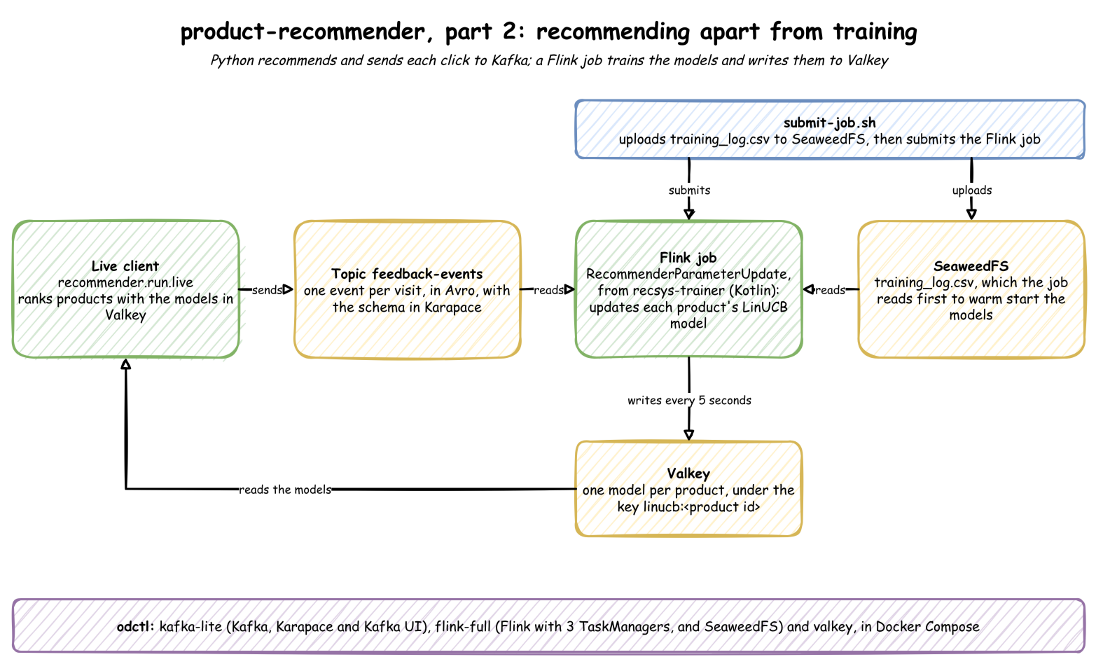
To move from prototype to production, we split the application into two distinct layers: Serving and Training.
- Python Client (Serving): A lightweight, stateless client responsible for inference. It fetches pre-calculated model parameters from Valkey, computes scores locally to make product recommendations, and captures user feedback.
- Kafka (Transport): Buffers feedback events asynchronously, decoupling the speed of serving from the speed of training.
- Flink (Training): A stateful streaming application. It consumes feedback events, updates the model parameters (LinUCB matrices $A$ and $b$), and pushes the inverted matrices back to Valkey.
- ❗ Unlike Part 1, where training relied on
MABWiser, here it is performed via explicit matrix operations.
- ❗ Unlike Part 1, where training relied on
- Valkey (Model Store): Stores the latest model parameters ($A^{-1}$ and $b$) for low-latency access by the client.
- ❗ Valkey is a fork of Redis and speaks the same wire protocol, so the client still uses
redis-pyand the Flink sink still uses Jedis.
- ❗ Valkey is a fork of Redis and speaks the same wire protocol, so the client still uses
📂 Source Code for the Post
The source code for this post is available in the product-recommender folder of the benchtop GitHub repository. It is one of the Benchtop projects, which run locally from a fresh clone.
Flink Application Design
The Flink job (recsys-trainer) ties these concepts together using a few specific patterns.
Stateful Model Training
The core challenge in distributed online learning is managing state. The LinUCBUpdater function in the Flink trainer acts as the system’s memory. It implements a disjoint LinUCB model, meaning it maintains a completely independent set of matrices for each unique product.
❗The matrices are used to calculate scores for making recommendations.
Each feedback event carries the visit’s context vector $x$: $d = 15$ numbers, the user’s 10 features and the 5 time flags from Part 1. For each product_id, Flink maintains two pieces of state in RocksDB:
- Matrix $A_a$ ($d \times d$): The sum of $x x^T$ over the contexts product $a$ was shown in, plus $\lambda I$. It tracks Exposure, recording how many times specific user contexts (e.g., “Morning Users” or “Weekend Users”) have been seen for a specific product.
- Vector $b_a$ ($d \times 1$): The sum of $r x$, the accumulated reward. It tracks Success, recording which features actually led to a click.
The matrix $A$ is initialized as a scaled identity matrix $A_0 = \lambda I$, with $\lambda = 1$, to ensure invertibility and to encode an initial prior of uniform uncertainty across feature dimensions.
When a feedback event arrives for product $a$ (context $x$, reward $r$: 1 for a click, 0 for none), Flink performs the updates:
- Update A: $A_a \leftarrow A_a + x x^T$. The outer product $x x^T$ makes $A_a$ larger along the observed feature directions. As similar contexts repeat, $A$ grows in those directions, reflecting increased confidence.
- Update b: $b_a \leftarrow b_a + r x$. If the user clicked ($r=1$), we add their feature vector to $b$, reinforcing that preference pattern.
The updated $A$ and $b$ are stored immediately in Flink keyed state (backed by RocksDB). With checkpointing enabled, this state is durably persisted and recovered in case of failure.
Optimization 1: Inversion on Write
To generate a score, we need the inverse matrix $A^{-1}$, which is computationally expensive. If we performed this inversion inside the Python client for every recommendation request, latency would increase significantly. Instead, the Flink training job periodically loads $A$ from state, factorizes it using LU decomposition, computes $A^{-1}$, and stores the inverse in Valkey. Because the contextual feature dimension in this demo is small, recomputing the inverse periodically remains efficient while keeping the serving layer lightweight.
Optimization 2: Batched Updates
In a high-traffic environment, a popular product might receive thousands of clicks per second. Inverting the matrix and writing to Valkey for every single click would be inefficient.
To solve this, we use Flink timers to buffer updates. The model state ($A$ and $b$) is updated immediately for every event, while the expensive inversion and Valkey write are triggered periodically (e.g., every 5 seconds). This drastically reduces CPU load and network traffic while keeping the model fresh.
Scalable Inference Logic
The Python client (recommender/run/live.py) is responsible for ranking items. It uses the Upper Confidence Bound (UCB) formula to balance exploiting known good items and exploring uncertain ones.
For a given user context vector $x$ and product $a$, the score is calculated as:
$$ \text{Score}a = \underbrace{x^T \theta_a}{\text{exploitation}} + \underbrace{\alpha \sqrt{x^T A_a^{-1} x}}_{\text{exploration}}, \quad \text{where } \theta_a = A_a^{-1} b_a $$
Prediction ($x^T \theta_a$)
This is the standard Linear Regression prediction. It asks: “Based on historical data, what reward should we expect from this user?” It is a linear estimate, not a probability. If the user matches features stored in vector $b$ (features that previously led to clicks), this term is high.
Exploration ($\alpha \sqrt{x^T A_a^{-1} x}$)
- Familiar User: If we have seen this user type many times, the matrix $A$ accumulates repeated contributions of $x x^T$. This increases the magnitude of $A$ in those feature directions. Because the exploration term depends on $x^T A^{-1} x$, a larger $A$ leads to a smaller quadratic form, shrinking the confidence bound. The model therefore relies more on exploitation.
- Cold Start: If we have rarely (or never) observed this feature pattern, $A$ remains close to its initial regularized identity matrix. After inversion, these directions yield larger values of $x^T A^{-1} x$, increasing the confidence bound and encouraging exploration to reduce uncertainty.
- ❗ $\alpha$ is a hyperparameter and it is set to 1.0, the value used in Part 1.
Hybrid Source for Warm Start
Contextual bandits suffer from the “Cold Start” problem. To mitigate this, we implement a Hybrid Source.
- File Source: Reads the historical CSV (
training_log.csv) generated in Part 1 to bootstrap the model state. - Kafka Source: Automatically switches to the live
feedback-eventstopic once the historical data is processed.
Custom Valkey Sink
We implement a custom Sink using the Sink V2 API and Jedis. This allows us to perform efficient SET operations to update the model parameters in Valkey directly from the Flink stream. Because each update overwrites the full parameter vector, repeated writes remain logically safe under at-least-once delivery semantics. Besides, because the upstream LinUCBUpdater batches the emissions, this sink receives highly aggregated model updates, preventing Valkey from being overwhelmed by write operations.
Recommender Simulation Design
To validate the architecture without live user traffic, we designed a Python client (recommender/run/live.py) that simulates the entire lifecycle of a recommendation request. This script plays two roles simultaneously: it acts as the Recommendation Service (serving predictions) and the User (providing feedback).
Serving Logic
In a production environment, this logic would live in a high-performance API. For this simulation, the Python client:
- Context Generation: Creates a synthetic user profile (Age, Gender) and derives key temporal features (e.g., Morning, Weekend) from a simulated timestamp to form the full context.
- Model Retrieval: Fetches the latest LinUCB parameters ($A^{-1}$ and $b$) for all active products directly from Valkey.
- Scoring and Ranking: Calculates the UCB score for every product, ranks them in descending order, and returns the top 5 highest-scoring items as the recommendation set.
Feedback Generation
To prove the model is learning, the simulation follows the same “Ground Truth” logic used in Part 1:
- Morning Routine: Users click “Drinks & Desserts” (Coffee) between 6 AM and 11 AM.
- Weekend Treats: On Saturdays and Sundays, users prefer “Pizzas” or “Burgers.”
- Price Sensitivity: Users under 25 avoid expensive items.
If any of the recommended top 5 items matches the user’s current context (e.g., showing a Latte on a Tuesday morning), the script generates a Reward (1). Otherwise, it generates no reward (0). This feedback is serialized to Avro and produced to Kafka, completing the loop.
Environment Setup
We use odctl to orchestrate the infrastructure (Kafka, Flink, Valkey) and Gradle to build the Kotlin application. odctl is a CLI that launches a local open data stack from a single command, resolving the dependency, networking, and connector wiring between engines on our behalf.
Prerequisites
odctl is installed alongside the other Python dependencies in requirements.txt, so the Part 1 environment already covers it. It needs Docker running, ideally with 8GB or more allocated.
1git clone https://github.com/jaehyeon-kim/benchtop.git
2cd benchtop/product-recommender
3
4uv python install 3.11
5uv venv --python 3.11 venv
6source venv/bin/activate
7uv pip install -r requirements.txt
Every command from here on runs from the product-recommender folder, as in Part 1.
Build and Launch
We bootstrap the environment by generating training data, building the Flink JAR, and launching the cluster.
❗ You do not need Kotlin or Gradle installed locally. The ./gradlew script handles all build dependencies, though it does require a JDK 17 toolchain.
1# Generate Bootstrap Data (skip if already done in Part 1)
2python -m recommender.run.prepare
3
4# Build Flink Application (Shadow Jar)
5(cd recsys-trainer && ./gradlew shadowJar)
6
7# Launch Kafka, Flink and Valkey
8odctl up kafka-lite flink-full valkey
Dependencies resolve themselves: flink-full quietly pulls in PostgreSQL, SeaweedFS (S3), and the Iceberg REST catalog before starting the compute engines. Run odctl ps --all to see everything that came up.
| Service | URL |
|---|---|
| Flink JobManager UI | http://localhost:8082 |
| Kafka UI | http://localhost:8086 |
| SeaweedFS (S3) file browser | http://localhost:8889 |
| Schema Registry (Karapace) | http://localhost:8081 (REST API, no UI) |
Submitting the Flink Job
odctl provides a Flink session cluster rather than running the job in application mode, so the JAR is submitted to the already-running cluster:
1./submit-job.sh
The script does three things: it uploads training_log.csv to SeaweedFS, copies the fat JAR into the JobManager container, and calls flink run -d.
The bootstrap CSV goes to object storage rather than a bind mount because Flink’s split enumerator runs on the JobManager while the readers run on the TaskManagers. With three TaskManagers, a local file path would need to exist in four separate containers.
Live Recommender Simulation
Once the infrastructure is running, Flink will first process the historical events to warm up. Once the historical processing is complete, we can run the Python client to simulate live traffic.
To visualize the system in action, open two terminals.
Terminal 1: Client
Run the Python script. It acts as the user, receiving recommendations and sending feedback (clicks) to Kafka.
1python -m recommender.run.live
Terminal 2: Trainer
Watch the Flink TaskManager logs. You will see the application reacting to the events sent to the feedback-events topic in real-time. The job’s six tasks need only six of the 15 slots, so Flink may place them on two of the three TaskManagers. Count each one’s writes first, then follow one with a count above 0:
1for tm in a b c; do echo "taskmanager-$tm: $(docker logs flink-taskmanager-$tm 2>&1 | grep -c 'Updated model')"; done
2docker logs flink-taskmanager-b -f
Result
You will see a series of feedback events generated by users on the left-hand side. On the right-hand side, you can see the logs confirming that model parameters are being sent to Valkey in batches.
This confirms the closed loop: Read (Valkey) -> Act (Kafka) -> Learn (Flink) -> Write (Valkey).
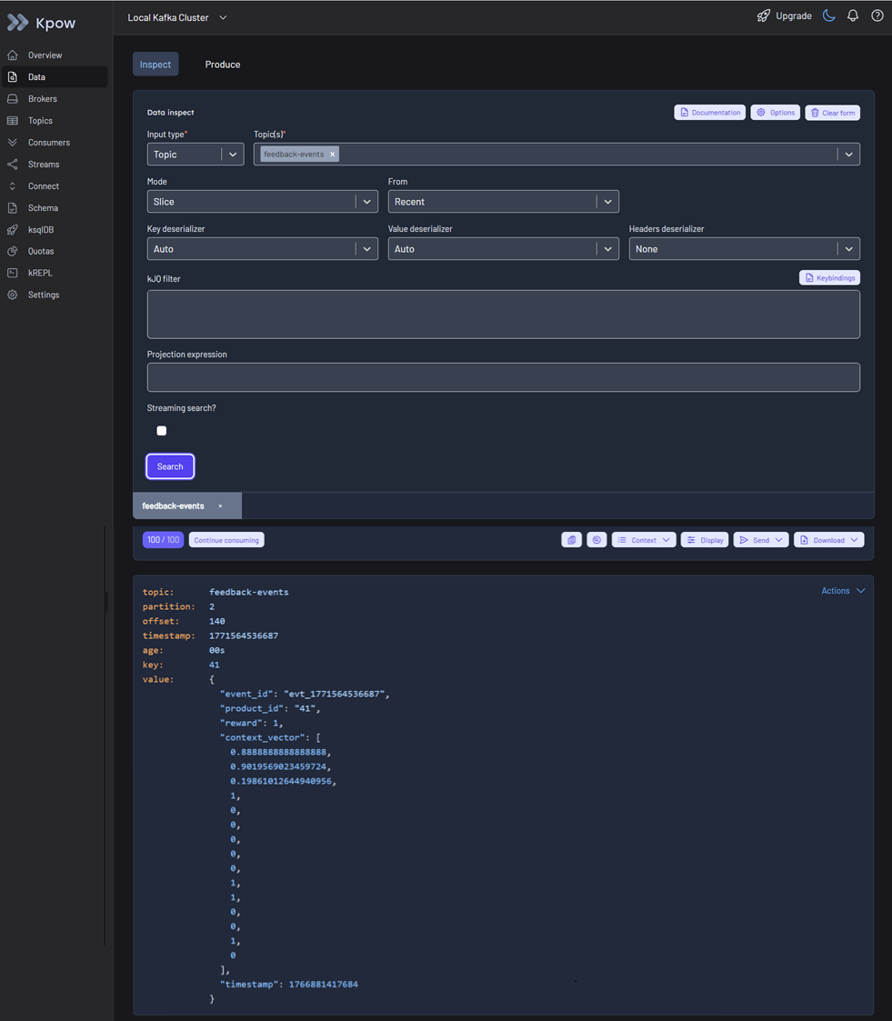
You can inspect feedback events on Kafka UI at http://localhost:8086.
Troubleshooting: the client defaults to
127.0.0.1rather thanlocalhost. On an IPv6-first host,localhostresolves to::1first, and the schema registry client fails outright with a connection reset instead of falling back to IPv4 the way the Kafka and Valkey clients do.
Teardown
To stop the cluster and remove resources:
1odctl down kafka-lite flink-full valkey
Add --volumes to also remove odctl-shared-deps, the named volume holding the downloaded connector JARs. The next odctl up then re-runs the init container to repopulate it.
Related posts
- Building a Real-Time Industrial Digital Twin with Apache Flink and Online Machine Learning - online machine learning on Flink and Kafka for an industrial digital twin, with drift detection and a shadow mode router
Conclusion
Traditional recommendation systems such as Collaborative Filtering rely on long-term interaction history and often treat user preferences as static. As a result, they struggle to incorporate immediate context, missing situational shifts like a user preferring coffee in the morning but pizza in the evening.
To overcome this, we use Contextual Multi-Armed Bandits (CMAB), an online learning approach that balances exploitation and exploration using real-time contextual signals. While our Python prototype in Part 1 validated the concept, it was not built for scale.
We then evolved it into a production-ready event-driven architecture: Kafka streams feedback events, Flink handles distributed stateful training, and Valkey serves precomputed parameters for low-latency inference. This design enables horizontal scalability and real-time adaptation to user behavior.


Comments