Output Analysis
A simulation run gives numbers, and a number from one run is a sample, not the answer. Output analysis is the work of turning runs into an answer with a stated precision. This page explains the ideas, and the tutorials and User Guide pages named below apply them to the packing shop and show the commands.
It follows the treatment of output analysis for a single model in Banks, Carson, Nelson and Nicol, Discrete-Event System Simulation, chapter 11, and the output-analysis pitfalls in Law, "Twenty-Three Critical Pitfalls in Simulation Modeling and How to Avoid Them" (Winter Simulation Conference, 2024). We read the chapter through lecture notes on it and the paper through its published text. The explanations are our own.
Terminating or Steady State
First decide which question the study asks. A terminating run ends at a time or an event the system has by nature, and starts from conditions the system really has. A shop that opens empty and closes at the end of the day is terminating: the day's answer is the answer. A steady-state study asks how a system behaves in the long run, after the effect of its starting conditions has gone. The same model can be either, because the choice depends on the question and on the system, not on the model.
The two ask for different handling of the start of the run and of its length:
- Terminating: the start is part of the answer. Run the real opening state, run to the real closing event, and use replications to measure the spread.
- Steady state: the start is a distortion. Leave out a warm-up, and run long enough that the rest represents the long run.
The busy hour of Trusting Results is treated as steady state, because the question is what the shop's waits usually are. End Conditions treats the shop as terminating: orders stop at 3,600 seconds and the question is what happens to the work still in the shop.
One Run Starts Empty
A run starts with an empty shop, and the first orders find every packer free. Their waits are shorter than the waits of the hour as a whole, so the mean wait of a run is biased low by its start. Look at the diagram for the two parts of a run: in the warm-up the shop fills from empty and the queue has not settled, so it is left out of the statistics, and the measured period, once the queue has settled, is what the statistics cover.
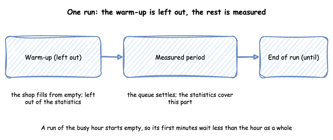
A warm-up is a time at the start of a run whose observations are discarded. In desflow the run's warmup resets every statistic once at that time, as Run Length and Statistics describe.
Choose the warm-up from evidence, not from habit. Plot a running statistic from the start of the run, such as the queue length or the mean wait so far, for several seeds, and pick a time after which they all move up and down with no trend. Law's paper shows a plot made with Welch's method for this, in which the warm-up is the time after which the average has levelled off, and advises choosing it conservatively. Compare a few candidate cutoffs as well: run the replications with each, and take the shortest after which a longer warm-up no longer moves the mean by more than its half-width. Trusting Results does it for the shop: the mean wait so far climbs for about a minute and a half and then wanders, so the warm-up is 2 minutes. For the busy hour it moves the mean wait of one run only from 1.382 to 1.381 seconds, because an hour is long enough that its first minutes hardly count. A shorter run, or one that starts far from the usual state, needs the warm-up much more.
A warm-up is not a fix for a model that never settles. If utilisation is 1 or more, there is no steady state, and no warm-up will find one, as Queueing Basics explains.
Replications
The waits of orders in one run follow each other: after a busy period, many orders in a row wait long. They are not independent samples, so the usual formula for the spread of an average, which assumes independent samples, gives an interval that is too narrow. Law lists this as a pitfall, along with treating one run as the truth.
Replications avoid the problem. Each replication is the same run with its own random stream, so it has its own mean wait, and gives one independent value of each statistic. The mean of those values is the estimate, and a 95% interval is the mean plus or minus t × s ÷ √n, where s is the standard deviation of the n values and t is the Student t quantile for n − 1 degrees of freedom. Look at the diagram for the flow from runs to one interval.
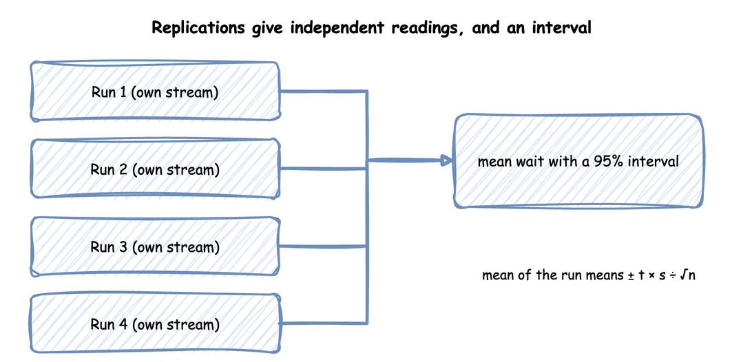
In the busy hour of the shop, 40 replications give a mean wait of 2.32 ± 0.20 seconds, and the run with the seed 42 alone measured 1.38 seconds, lower than any of the 40. One run would have given a confident and wrong answer. Trusting Results shows these runs, Replications describes the commands and the seeds, which are spawned from one seed so that the set repeats exactly, and Randomness and Seeds explains the streams.
How Many Replications
There is no fixed number that is enough. Decide the precision each output needs, such as a half-width within 10% of the mean, and run until the least precise output has it. In the shop, utilisation meets 10% with 5 replications, and the mean wait first meets it at 40, because waits vary far more from run to run than how busy the packers are. The half-width shrinks with √n, so a short run can suggest the number needed, and then the interval has to be read again, because the half-width is itself an estimate. Trusting Results shows the table.
A longer run is the other way to buy precision, and it has limits of its own: it reduces the effect of the start, but its mean is still one sample.
Which Orders a Reading Covers
A mean is over some orders, and the page that reports it should say which. At a fixed horizon, some orders have started and not finished, and the mean wait covers those that started. With a drain, every order admitted finishes, at the cost of running past the hour. In End Conditions the fixed horizon ends at 3,600 seconds with 2,436 orders started, 2,398 finished and 38 in the shop, and the drain ends at 3,656.4 seconds with all 2,436 finished.
The warm-up adds a third group, orders that were in the shop when the warm-up ended. An order that started before the warm-up ended and finished after it is counted as finished and in the wait and service times, with its whole wait, but not as started. Statistics has the table of which orders each count covers. Report the counts beside the means.
Comparing Designs
To tell whether a design is better, compare the designs with the same random numbers. Run each design with the same seeds, so that each pair of runs meets the same arrivals and the same service times, and take the difference seed by seed. The chance part partly cancels, so the interval on the differences is narrower than the interval an unpaired comparison of the same runs gives, as Comparing Designs uses it: a fourth packer cuts the busy hour's mean wait by 2.21 ± 0.31 seconds.
The check below shows the effect on 40 runs of the busy hour with 3 packers, 20 packing in 1.5 seconds and 20 packing in 1.45 seconds, with the same 20 seeds. It builds two intervals for the difference of the mean waits from the same runs: one paired by seed, and one that treats the designs as independent.
The difference is 0.69 seconds. The paired interval is ± 0.12 seconds and the unpaired one is ± 0.29 seconds, so pairing more than halves the interval here.
Pairing helps only when the designs use the random numbers in the same way. desflow gives each distribution a stream of its own, so adding a step to one design does not shift the numbers the shared steps draw. The comparison report lists any stream that only one design used, because draws from such a stream are not paired. Check that list before trusting a paired interval. Law names comparing designs without a sound statistical approach as a pitfall. The lecture notes on Banks et al. give the interval across replications the same form as the one above.
What to Report
State, for each answer:
- The question: terminating or steady state, and the period it covers.
- The warm-up, and the evidence for it.
- The number of replications and the seeds' source.
- Each output as a mean with its half-width, and the precision the decision needed.
- Which orders each count covers.
Readiness and Reporting lists what a report must contain.