Queueing Basics

A queue forms whenever work arrives faster than it can be served for a while, and the length of the wait depends on more than the averages. This page explains the few results of queueing theory that a simulation study uses, each with a run of the packing shop that checks it. The numbers on this page come from queueing_basics.py, which asserts every one of them.

The sources are the Wikipedia articles on Kendall's notation, Little's law, Kingman's formula and the Erlang C formula. The explanations and the checks are our own.

---

Parts of a Queue

A queueing model has arrivals, a queue, and one or more servers. In the shop these are the orders, the queue in front of the packers, and the packers. Look at the diagram for the three things a model must say: how far apart orders arrive, how long a packer takes, and how many packers there are.

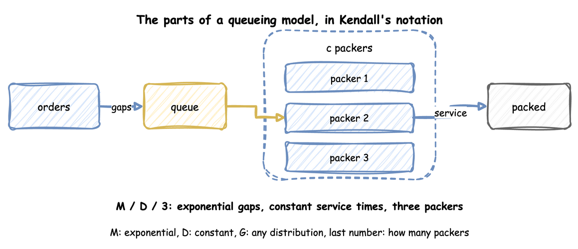
Kendall's notation writes these as arrivals/service/servers. M is an exponential distribution, D a constant one and G any distribution, and the last number is the count of servers. The shop's busy hour in Queues and Capacity is M/D/3. When a model leaves out the further terms, they have their defaults: the queue has room for any number of orders, the population that orders come from is unlimited, and orders are served in the order they arrive.

The measure that decides everything is utilisation, the share of time a server is busy: the arrival rate times the mean service time, divided by the number of servers. Below 1 a queue is stable and its length settles. At 1 or above, when the gaps or the service times vary, the queue grows without limit. Above 1 it grows in every case, even when the gaps and service times are constant. Queues and Capacity works this out for the shop.

---

Little's Law

Little's law says that, in a system that settles, the average number of orders in it equals the arrival rate times the average time an order spends in it: L = λ × W. It needs no assumption about the arrival or service distributions or about the order of service, and it holds for the queue alone, for the packers alone, or for both together.

Because it is so general, it is the first check on a model's statistics: the queue length, the arrival rate and the wait are measured separately, and they must agree. Here is the busy hour with three packers. The function runs the shop for 20,000 seconds and returns the arrival rate, the queue length with the mean wait, and the number in the shop with the mean time in the shop:

UNTIL = 20_000  # seconds, long enough that the start and end of the run hardly count


def little():
    """One run of the busy hour with 3 packers; returns L, lambda and W for the queue and the shop."""
    app = shop(exponential(1 / 1.8), constant(SERVICE), packers=3)
    app.run(until=UNTIL)
    r = app.env.stats.readings()
    arrival_rate = r["Shop.stats.flows.orders.started"] / UNTIL
    in_queue = r["Shop.stats.resources.packers.queue_length_avg"]
    in_service = 3 * r["Shop.stats.resources.packers.utilization_avg"] / 100
    wait = r["Shop.stats.tasks.pack_order.wait_mean"]
    service = r["Shop.stats.tasks.pack_order.service_mean"]
    return arrival_rate, (in_queue, wait), (in_queue + in_service, wait + service)

The shop it uses is built by this function, in which the arrival gaps and the service times are exponential or constant by choice:

def shop(arrival: dict, service: dict, packers: int) -> SimulationContext:
    """The shop with the given arrival gaps and packing times, and `packers` packers."""
    app = SimulationContext(sim_id="Shop", factor=0, random_seed=42)
    app.add_arrival("orders", **arrival)
    app.add_service("packing", **service)
    app.add_resource("packers", current_cap=packers, max_cap=10)
    app.with_stats("typical", interval=3600)

    @app.task(service_id="packing", resource_id="packers")
    def pack_order(task_id):
        return {"event_type": "order_packed"}

    @app.arrival_loop("orders")
    def order_generator(context):
        task_id = 0
        while True:
            order = yield context.wait_for_arrival("orders")
            context.spawn(pack_order(task_id, entity=order))
            task_id += 1

    return app


# Exponential gaps and times are the M of Kendall's notation, constant ones the D
def exponential(mean: float) -> dict:
    return {"dist": "exponential", "rate": 1 / mean}


def constant(mean: float) -> dict:
    return {"dist": "constant", "value": mean}

Run with exponential gaps of mean 1/1.8 s and constant(1.5) service, it prints:

arrival rate 1.782 orders per second
queue: L 3.417, lambda x W 3.417
shop: L 6.089, lambda x W 6.090

In both cases the two figures agree within 1%. For the whole shop, the number in service is the mean utilisation times the three packers. Checking and Validating uses this as a test of a model.

Utilisation can be checked the same way. The measured share of time the packers are busy must equal the arrival rate times the mean service time, divided by the number of packers:

def utilisation():
    """One run of the busy hour; returns utilisation from the formula and as measured."""
    app = shop(exponential(1 / 1.8), constant(SERVICE), packers=3)
    app.run(until=UNTIL)
    r = app.env.stats.readings()
    rate = r["Shop.stats.flows.orders.started"] / UNTIL
    return rate * SERVICE / 3, r["Shop.stats.resources.packers.utilization_avg"] / 100

formula, measured = utilisation()
print(f"utilisation {formula:.3f} from the formula, {measured:.3f} measured")
assert abs(formula - 0.891) < 0.0005 and abs(measured - formula) < 0.005

utilisation 0.891 from the formula, 0.891 measured

---

Waits Near Full Use

For an M/M/1 queue, which has exponential gaps and service times and one server, the mean wait in the queue has a closed form: utilisation ÷ (1 − utilisation) × the mean service time. With constant service times (M/D/1) it is exactly half. Look at how the bars grow faster than the utilisation: from 0.9 to 0.95 the wait more than doubles.

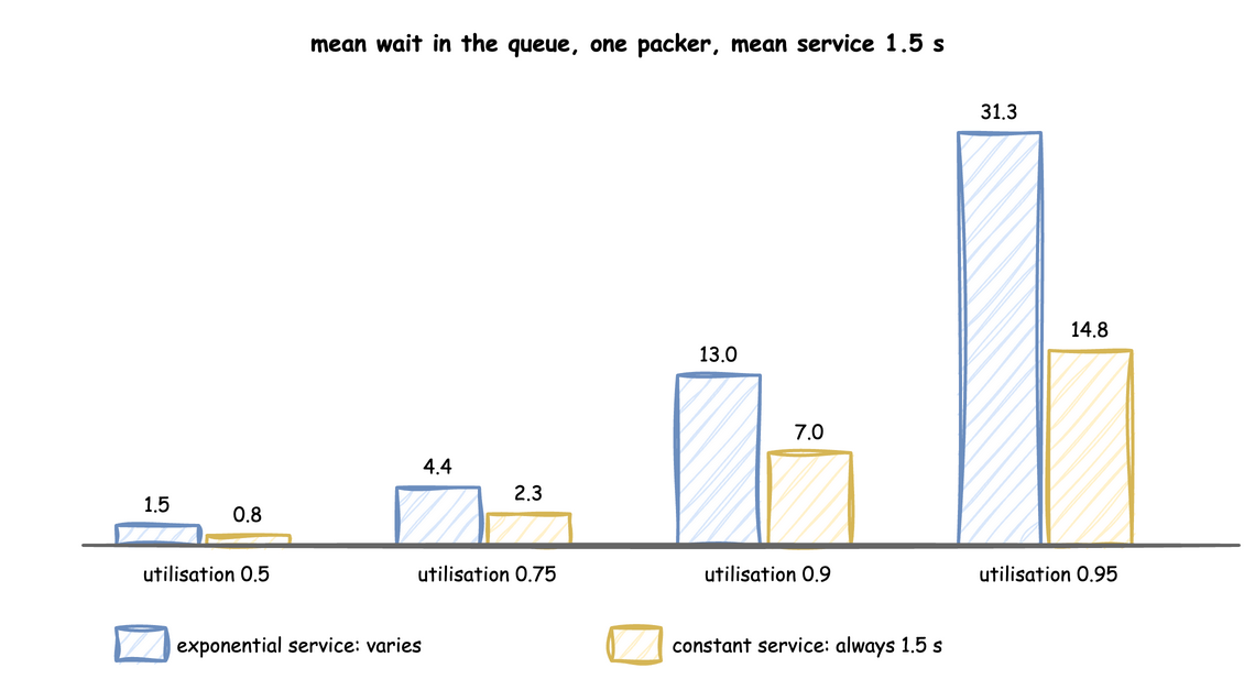
The formulas are short enough to write down and compute:

def mm1_wait(utilisation: float) -> float:
    """Mean wait in the queue of an M/M/1 queue: utilisation / (1 - utilisation) x service."""
    return utilisation / (1 - utilisation) * SERVICE


def erlang_c(units: int, load: float) -> float:
    """The share of arrivals that find all `units` busy, for a load in packers' worth of work."""
    last = load**units / math.factorial(units) / (1 - load / units)
    return last / (sum(load**k / math.factorial(k) for k in range(units)) + last)


def mmc_wait(units: int, arrival_rate: float) -> float:
    """Mean wait in the queue of an M/M/c queue: Erlang C divided by (c / service - lambda)."""
    return erlang_c(units, arrival_rate * SERVICE) / (units / SERVICE - arrival_rate)


def kingman_wait(utilisation: float, arrival_cv: float, service_cv: float) -> float:
    """Kingman's approximation of the mean wait in a one-server queue."""
    variability = (arrival_cv**2 + service_cv**2) / 2
    return utilisation / (1 - utilisation) * variability * SERVICE

utilisation 0.5: M/M/1  1.50 s, M/D/1  0.75 s
utilisation 0.75: M/M/1  4.50 s, M/D/1  2.25 s
utilisation 0.9: M/M/1 13.50 s, M/D/1  6.75 s
utilisation 0.95: M/M/1 28.50 s, M/D/1 14.25 s

A queue that is stable can still make orders wait a long time, so a design that only keeps utilisation below 1 is not enough. This is also why the run length matters: near full use, a run needs to be long before its mean wait settles, as Output Analysis explains.

---

Several Packers

With several packers sharing one queue, the wait depends on the chance that every packer is busy when an order arrives. For exponential gaps and service times (M/M/c) that chance is the Erlang C formula, and the mean wait in the queue is that chance divided by (c ÷ the mean service time − the arrival rate). The erlang_c and mmc_wait functions above compute it.

More packers cut the wait faster than the share of work each does. One packer at utilisation 0.8 makes orders wait 6 seconds. Three packers at the same utilisation make them wait about 1.6 seconds, because an order waits only when all three are busy. Both values come from the formulas, and the script prints them:

one packer at utilisation 0.8: 6.0 s
three packers at utilisation 0.8: 1.62 s

---

Variation Lengthens Waits

Real gaps and service times are rarely exponential. Kingman's approximation covers any distributions, for one server: the mean wait is utilisation ÷ (1 − utilisation) × (arrival variation² + service variation²) ÷ 2 × the mean service time, where variation is the standard deviation divided by the mean, so it is 1 for an exponential distribution and 0 for a constant one. With exponential gaps (variation 1) and constant service (variation 0) it gives half the M/M/1 wait, which is the M/D/1 result above.

The kingman_wait function above computes it. Variation in the gaps counts as much as variation in the service times. A model whose inputs are replaced by their averages shows no queue at all. Choosing Inputs measures how much the spread of an input matters. Common Mistakes lists the replacement among the errors that distort a result.

---

Check a Formula Against the Shop

Each formula above is checked with the shop. The function runs ten replications of a run, each leaving out its first 2,000 seconds, and returns the mean wait with its 95% half-width. Output Analysis explains why each run leaves out its start and why the interval comes from several runs.

def measured_wait(arrival: dict, service: dict, packers: int, until: int):
    """Mean wait over 10 runs, with its 95% half-width; each run leaves out its first 2,000 s."""
    result = replicate(
        lambda: shop(arrival, service, packers),
        10,
        seed=42,
        until=until,
        warmup=2000,
        measures=["tasks.pack_order.wait_mean"],
    )
    row = result.summary[0]
    return row["mean"], row["half_width"]

Each check passes when the formula lies within the interval:

for rho, figures in ((0.5, (1.50, 1.47, 0.06)), (0.75, (4.50, 4.46, 0.33))):
    arrival = exponential(SERVICE / rho)
    check(
        f"M/M/1 at {rho}",
        mm1_wait(rho),
        measured_wait(arrival, exponential(SERVICE), 1, 20_000),
        figures,
    )
check(
    "M/M/3 at 0.8",
    mmc_wait(3, 1.6),
    measured_wait(exponential(1 / 1.6), exponential(SERVICE), 3, 30_000),
    (1.62, 1.64, 0.06),
)
arrival = exponential(SERVICE / 0.75)
check(
    "M/D/1 at 0.75, Kingman",
    kingman_wait(0.75, 1, 0),
    measured_wait(arrival, constant(SERVICE), 1, 20_000),
    (2.25, 2.23, 0.14),
)

M/M/1 at 0.5: formula 1.50 s, runs 1.47 ± 0.06 s
M/M/1 at 0.75: formula 4.50 s, runs 4.46 ± 0.33 s
M/M/3 at 0.8: formula 1.62 s, runs 1.64 ± 0.06 s
M/D/1 at 0.75, Kingman: formula 2.25 s, runs 2.23 ± 0.14 s

The diagram names the busy hour M/D/3, which has no exact formula here. The check runs the shop as M/D/3 at arrival rate 1.8 and compares the runs with half the M/M/3 wait at this load:

# The busy hour is M/D/3: exponential gaps (M), constant service (D), three packers.
# The runs are compared with half the M/M/3 wait at this load.
check(
    "M/D/3 at 0.9, half the M/M/3 wait",
    mmc_wait(3, 1.8) / 2,
    measured_wait(exponential(1 / 1.8), constant(SERVICE), 3, 20_000),
    (2.04, 2.05, 0.13),
)

M/D/3 at 0.9, half the M/M/3 wait: formula 2.04 s, runs 2.05 ± 0.13 s

The runs (2.05 ± 0.13 seconds) agree with half the M/M/3 wait (2.04 seconds) at this load.

Kingman's formula is an approximation, and the script shows where it is not exact. For constant gaps of 2 seconds and exponential service (D/M/1) at utilisation 0.75:

mean, half_width = measured_wait(
    constant(SERVICE / 0.75), exponential(SERVICE), 1, 20_000
)
kingman = kingman_wait(0.75, 0, 1)
print(
    f"D/M/1 at 0.75: Kingman {kingman:.2f} s, runs {mean:.2f} ± {half_width:.2f} s"
)

D/M/1 at 0.75: Kingman 2.25 s, runs 1.78 ± 0.09 s

The formula lies outside the interval of the runs. It is accurate near full use and for the cases above, and a rough guide elsewhere.

---

What to Take From It

• Compute utilisation first. At 1 or above, the answer is more capacity.
• Check a model's statistics with Little's law before trusting any result.
• Expect long waits near full use, and longer ones when gaps or service times vary.
• Use the formulas to check a model on the cases they cover. They do not replace the simulation, which handles the cases they cannot: several resources, priorities, breakdowns and changing demand.